Project 2: Introduction to the background and theory

David L Miller

BioSS/UKCEH

Thomas Cornulier

BioSS

Problem specification

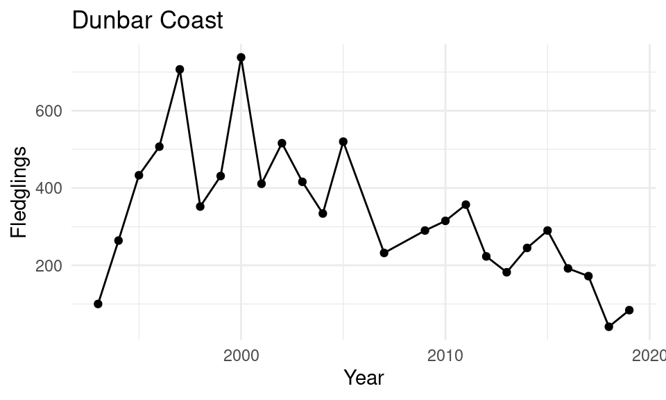
Kittiwakes: how are they doing?

• Measure: “breeding success”
  • Number of fledglings per year
  • (From “apparently occupied nests”)

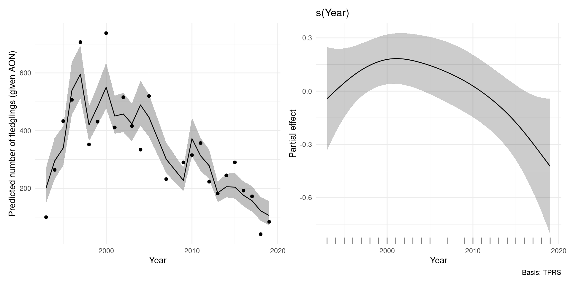
A basic model

Breeding success is a function of time

\[ \texttt{Fledg}_t = \exp\left(\beta_0 + \texttt{AON}_t + s(t)\right) \]

where \(\texttt{Fledg}_t \sim \text{Tweedie}(\phi, p)\).

• \(t\) indexes years
• \(\beta_0\) is an intercept
• \(\texttt{Fledg}_t\) is the number of fledglings
• \(\texttt{AON}_t\) number of apparently occupied nests
• \(s(t)\) smooth of year

In R…

library(mgcv)
m_t <- gam(Fledg ~ offset(log(AON + 1)) + s(Year, k=20),
                     data= kit1_fi, family= tw())

That’s all well and good, but…

We need to do some ecology?

• We want to know why
• What influences this?
  • (Remotely sensed) covariates?
    • sea surface temperature
    • lesser sandeel Ammodytes marinus distribution

Source: https://commons.wikimedia.org/wiki/File:Tobiasz.JPG

Sand eels

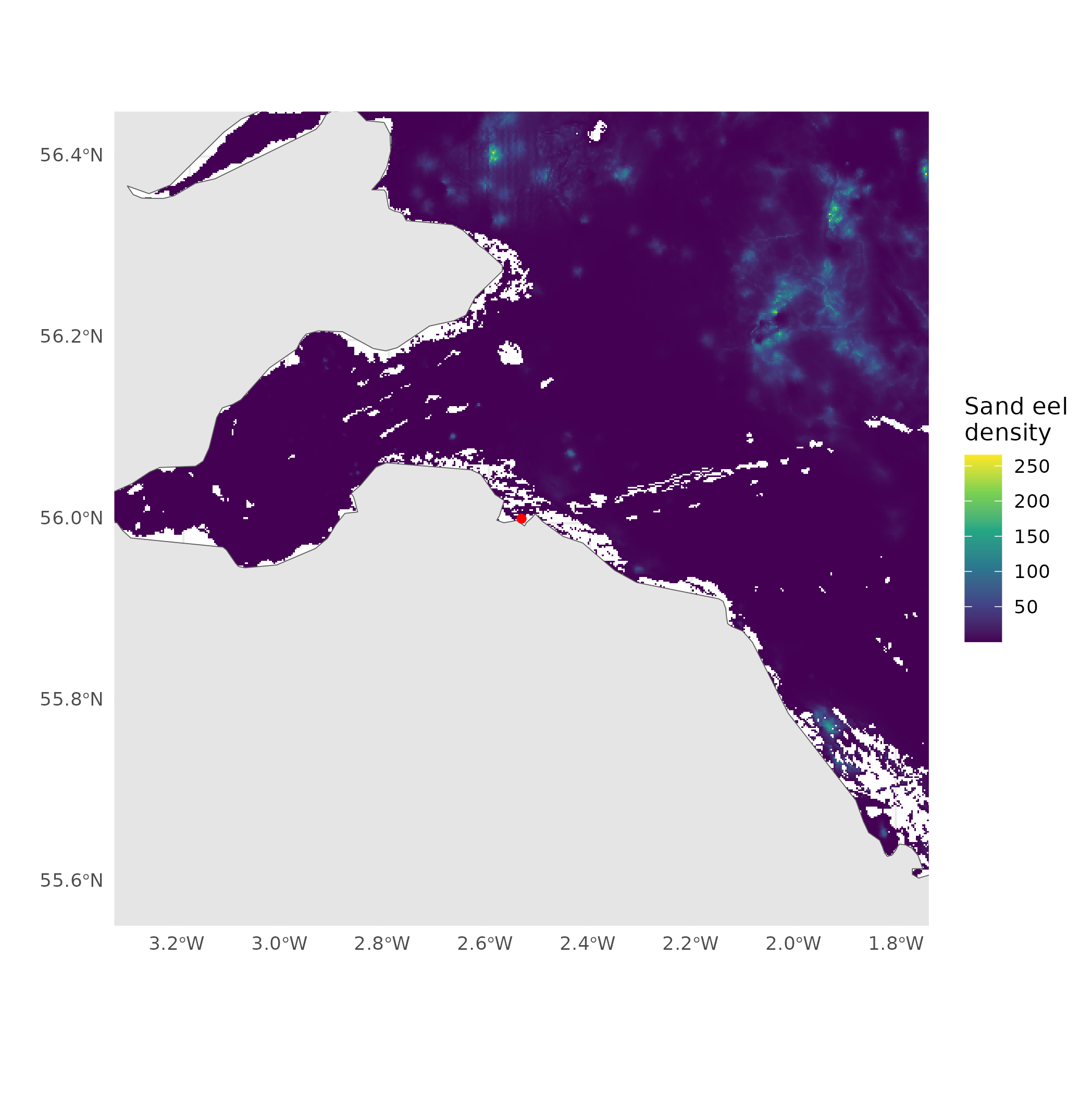
• We have a map of sandeel distribution
• We can just “plug-in” values, right?

Langton, R., Boulcott, P. and Wright P.J. (2021) A verified distribution model for the lesser sandeel Ammodytes marinus. Marine Ecology Progress Series.

What does that look like?

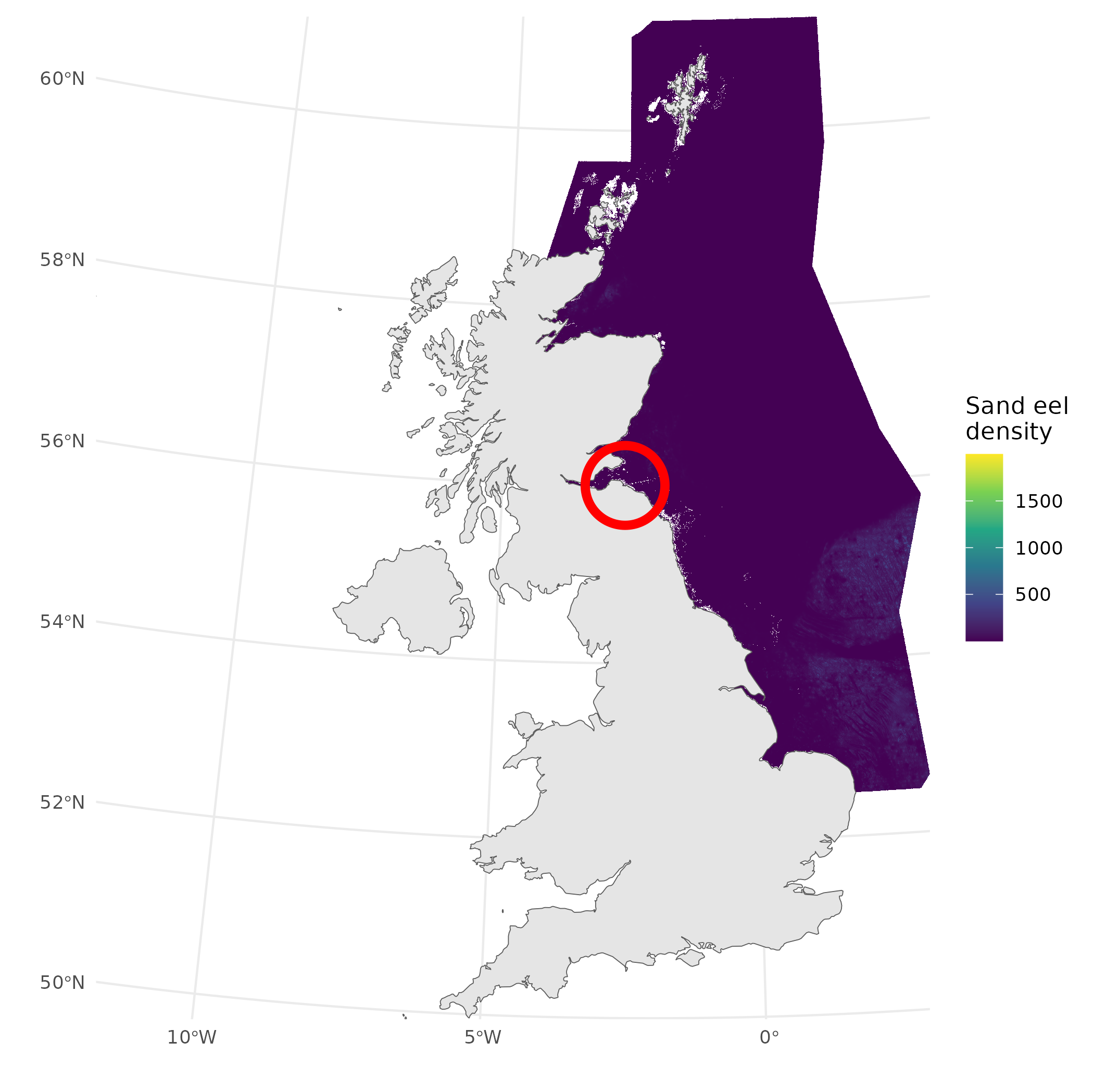
(zoom and enhance)

• Which value should we take?
  • Closest?
  • Average?
    • At what distance?
• What does the literature say?

Let’s simplify that

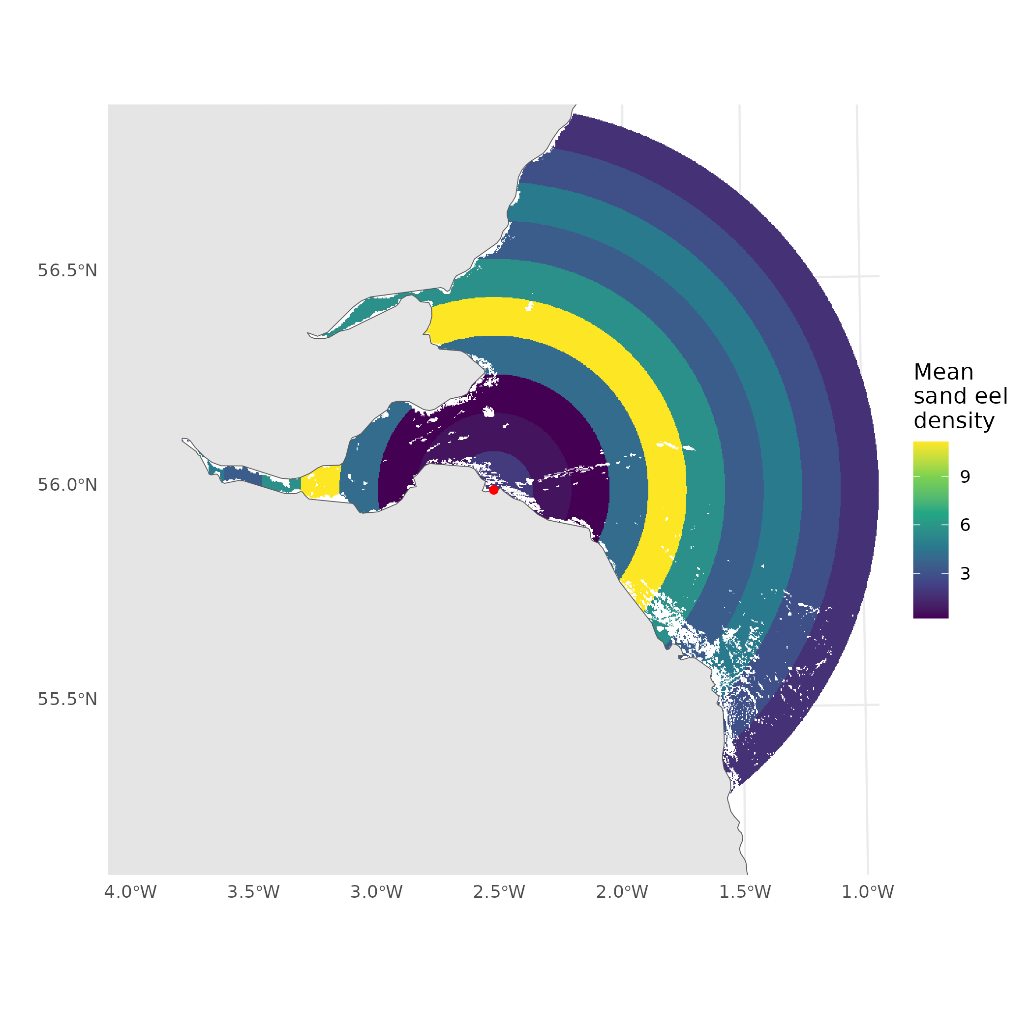
• We know a little about foraging distance
• Rings (annuli 🧐)
  • Simplifying assumption
  • 10km wide, up to 100km away

How can we build a model for this?

New problem specification

• We now have 10 values (10 rings) of sandeel density
• We don’t know which one is “right”
  • 👻 maybe more than one is right 👻
• How can we include 10 values in the model?

Approaches from literature

• Put all the covariates in the model
  • eel1 + eel2 + ...
  • Colinearity?
  • Independence??
• Fit a LOT of models
  • Which is best (by AIC?)?
  • Is this a good idea? (No)

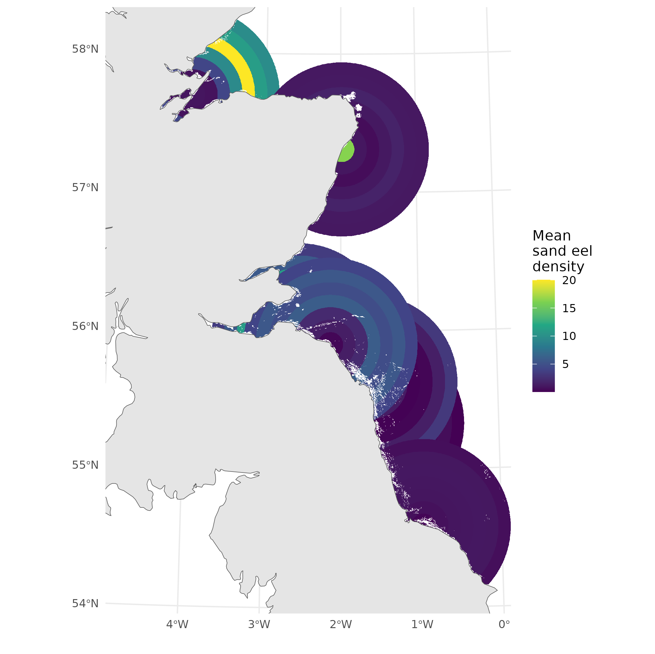
🧠 Extending to multiple sites

• Can we learn something about general kittiwake ecology?
• What can we generalize?
• What can we say about overall trends?

What do we really want here?

• Some average over the rings, but how do we weight them?
• What if we could weight while fitting?
  • more efficient use of information
  • (hint: that’s what we’ll do)

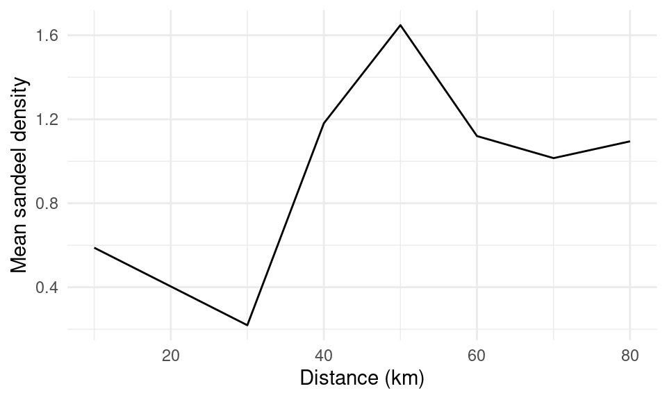
What does that data actually look like?

• (Restricting to 80km radius)
• We have 8 data points
• For one site
• Can we get the model to select which one(s) are useful?
  • (Yes)

Weighted averaging

• To estimate a weighted mean:

\[ \sum_j w_j x_j \]

• what if \(w_j\) and \(x_j\) are functions?

\[ \sum_j w(z_j) x(z_j) \]

Weighted averaging in a GAM

\[ \sum_j w(z_j) x(z_j) \]

• \(w(z_j)\) is a smooth we estimate

• \(x(z_j)\) is the sandeel density

• \(z_j\) are the distances

• \(\Rightarrow\) weighted average of sandeel density over the distances

  • where we estimate the weighting

Let’s do that…

Enter signal regression

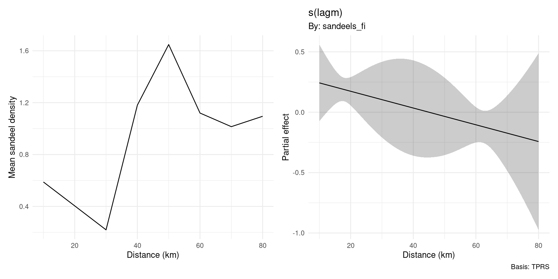
Signal regression, in maths

\[ \texttt{Fledg}_t = \exp\left( \beta_0 + \texttt{AON}_t + s(t) + \sum_j w(d_j) e(d_j) \right) \]

• Everything else as before but now an extra weighted sum
• \(d_j\) are the distance “lags” we have sandeel density at
• \(w(d_j)\) is our smooth of distance
• \(e(d_j)\) is the value of sand eel density at distance \(d_j\)

Signal regression, in R

m_t_e <- gam(Fledg ~ offset(log(AON + 1)) +
                     s(Year, k=20) +
                     s(lagm, by=sandeels_fi, k=6),
             data= kit_sub, family= tw())

“estimate a smooth (the weighting) of lagm (distances) and multiply by the sandeel density at that distance”

What does that data look like?

• lagm and sandeels_fi are nrow(kit_sub) \(\times\) (number of distances) matrices

head(lagm)

     [,1] [,2] [,3] [,4] [,5] [,6] [,7] [,8]
[1,]   10   20   30   40   50   60   70   80
[2,]   10   20   30   40   50   60   70   80
[3,]   10   20   30   40   50   60   70   80
[4,]   10   20   30   40   50   60   70   80
[5,]   10   20   30   40   50   60   70   80
[6,]   10   20   30   40   50   60   70   80

head(sandeels_fi)

          [,1]      [,2]    [,3]     [,4]     [,5]     [,6]    [,7]     [,8]
[1,] 0.5881714 0.4039171 0.21924 1.180914 1.648092 1.119965 1.01492 1.094924
[2,] 0.5881714 0.4039171 0.21924 1.180914 1.648092 1.119965 1.01492 1.094924
[3,] 0.5881714 0.4039171 0.21924 1.180914 1.648092 1.119965 1.01492 1.094924
[4,] 0.5881714 0.4039171 0.21924 1.180914 1.648092 1.119965 1.01492 1.094924
[5,] 0.5881714 0.4039171 0.21924 1.180914 1.648092 1.119965 1.01492 1.094924
[6,] 0.5881714 0.4039171 0.21924 1.180914 1.648092 1.119965 1.01492 1.094924

Recap

We can use signal regression (aka scalar-on-function regression) to make weighted averages of “functional” data.

We assume that sandeel density is a function of distance from colony.

We estimate the weighting needed during fitting.

Adding complication: more sites

Adding sites

• Want to look at colony status over multiple sites
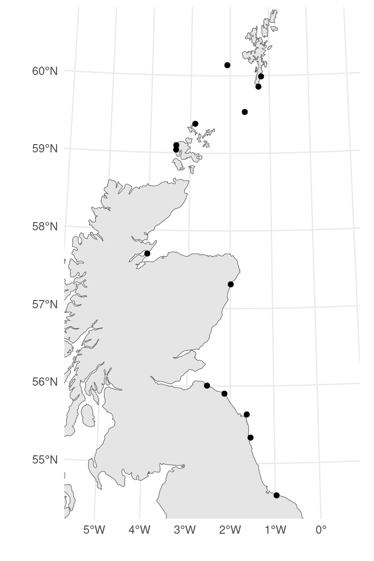
• Let’s include data from 14 sites
  • (where we have the sandeel data)

Adding site-specific effects (maths)

\[\begin{equation} \texttt{Fledg}_{ti} = \exp\left( \beta_0 + \texttt{AON}_{ti} + s(t) +\\ \qquad \sum_j w(d_j) e_i(d_j) + \texttt{Site}_i \right) \end{equation}\]

• (extra index \(i\) for site)
• AON is now site (\(i\)) and time (\(t\)) specific
• site random intercept \(\texttt{Site}_i\)

• sandeel density per site \(e_i()\)
  • but still looking for common distance smooth!

Adding site-specific effects (R)

m_t_e_s <- gam(Fledg ~ offset(log(AON + 1)) +
                       s(Year, k=20) +
                       s(lagm, by=sandeels_fi, k=6) +
                       s(Site, bs="re"),
               data= kit2, family= tw())

What does that look like?

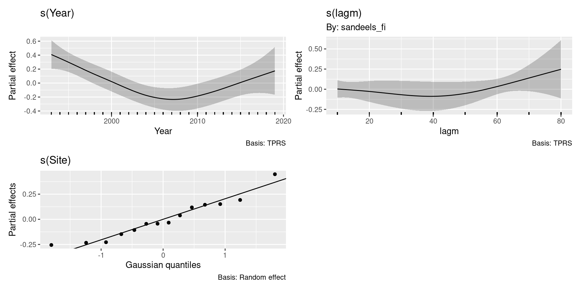
Some things to think about here

• How reasonable is this model?
• Do we expect that the distance effect is the same for all sites?
• Should we have a spatial effect rather than site random effect?
• Are there other plausible models?

But we need to keep going…

More complicated example using SST

Sea surface temperature

• How should we include SST in the model?
• Expand our model like this?

\[ \texttt{Fledg}_t = \exp\left(\beta_0 + \texttt{AON}_t + s(t) + s(\texttt{SST}_t)\right) \]

• Easy, right?

Things are never easy…

• We have weekly SST
• We have SST on a 10km grid
• Which one is important?

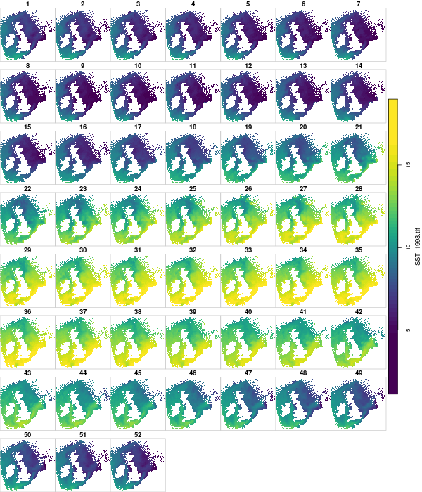
Going back to just Dunbar

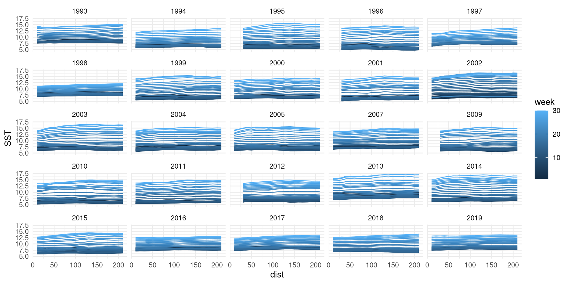
That’s a lot

We can do the same trick though!

• Let’s simplify again using rings
• Two lags: time and distance
• Let’s do all sites
  • and let the smooth vary by site

What can we get to?

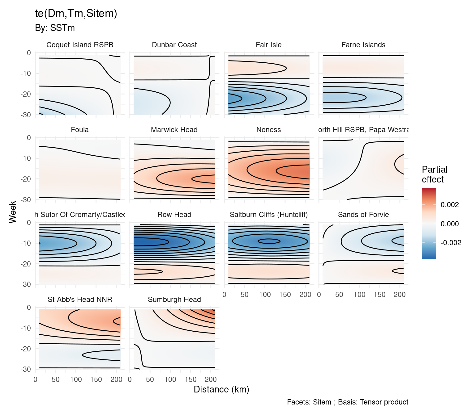
What just happened?

No, really

• We made another average but it’s really fancy now
• For a given \(\texttt{Site}\)

\[ \sum_j \sum_k w(d_j, t_k, \texttt{Site}) \texttt{SST}(d_j, t_k, \texttt{Site}) \]

• \(w(d_j, t_k, \texttt{Site})\) is a smooth we estimate
• \(\texttt{SST}(d_j, t_k, \texttt{Site})\) is the SST
• \(d_j\) are the distances
• \(t_k\) is the week

How do we build \(w(d_j, t_k, \texttt{Site})\)

• Let’s start with just making a smooth of 2 variables
  • \(s(x, y)\)
  • but \(x\) and \(y\) are on different scales
• Tensor products!

Tensor what?

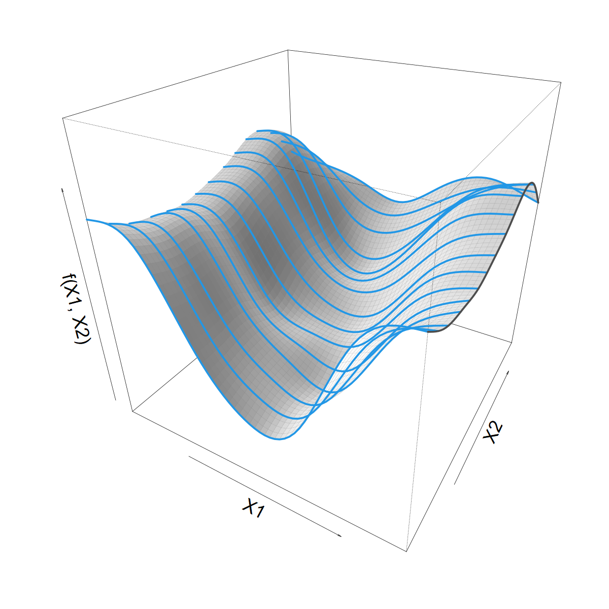
Looking for a smooth function \(f(X1, X2)\)

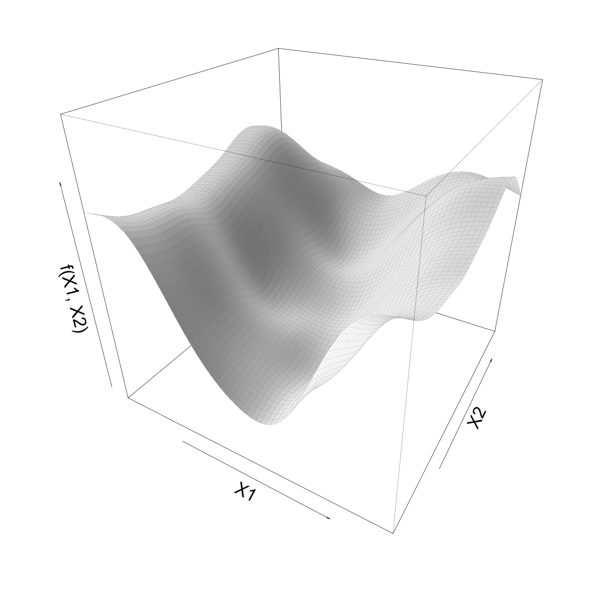
Smoothing over \(X1\)

• Let’s start with a standard 1D smoother

\[ s(X1) = \sum_k \beta_k b_k(X1) \]

• Built from basis functions \(b_k(X1)\)
• With coefficients \(\beta_k\) (“weights”)

Smoothing over \(X1\)

• Let’s start with a standard 1D smoother

\[ s(X1) = \sum_k \beta_k b_k(X1) \]

• Built from basis functions \(b_k(X1)\)

• With coefficients \(\beta_k\) (“weights”)

• We want to let \(s(X1)\) vary with \(X2\)

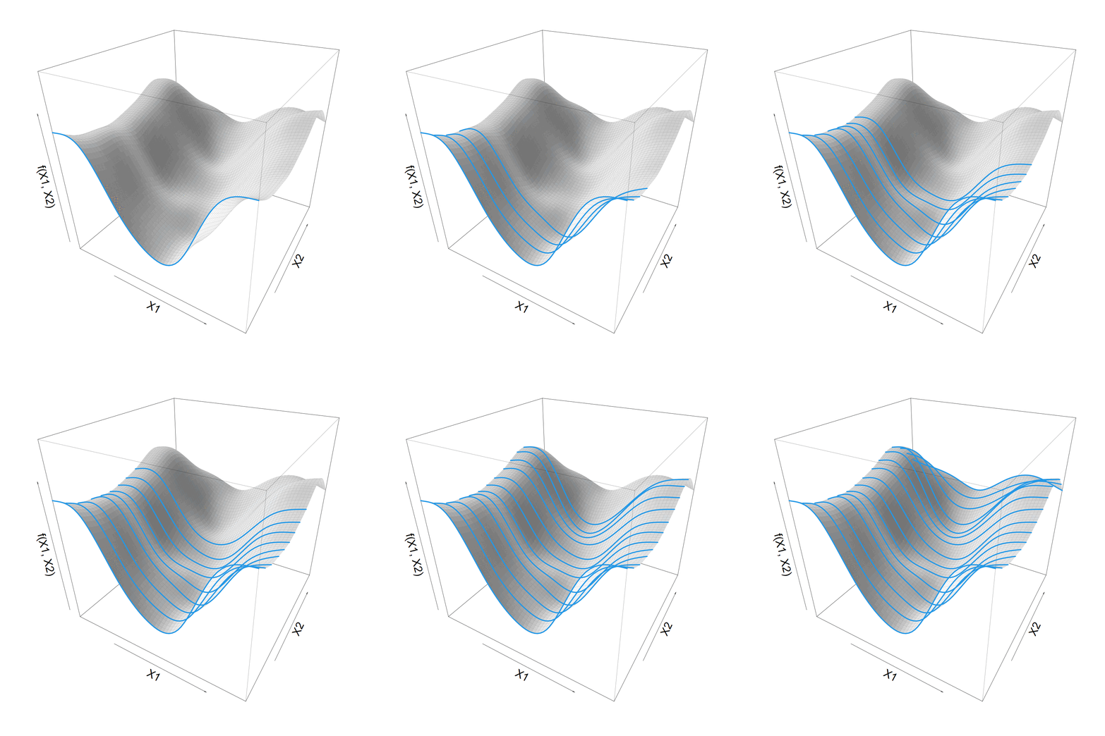
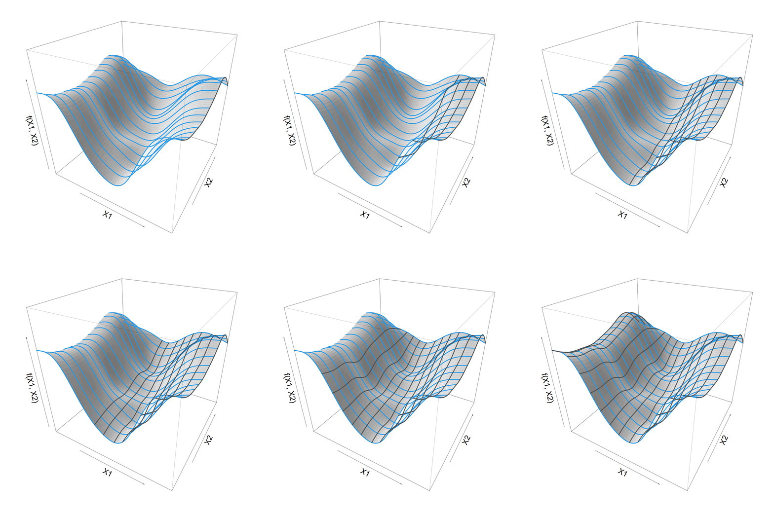
Making \(s(X1)\) vary smoothly with \(X2\)

\[ s(X1) = \sum_k \beta_k b_k(X1) \]

\(\beta_k\) now 1D smooth function of \(X2\)

\[ \beta_k(X2) = \sum_j \alpha_{jk} a_j(X2) \]

Making \(s(X1)\) vary smoothly with \(X2\)

\[ s(X1) = \sum_k \beta_k b_k(X1) \]

\[ \beta_k(X2) = \sum_j \alpha_{jk} a_j(X2) \]

\[ f(X1,X2) = \]

\[ \sum_j \sum_k \alpha_{jk} a_j(X2) b_k(X1) \]

What about that Site bit?

• We can go from 2 to more dimensions
• Site is special because it’s a factor
• but we can tensor splines and random effects
• Generates a copy of the smooth for each Site
  • smoothing towards each other
• (see also Fergus’ talk!)
• This is a kind of hierarchical GAM

So, in R?

Setting-up the model in R

m_dts <- gam(Fledg ~ offset(log(AON + 1)) + Year + Site +
                 te(Dm, Tm, Sitem, by= SSTm, k= c(4, 4, 14),
                    bs= c("tp", "tp", "re")),
             data= kit2,
             family=tw(), method= "REML")

Setting-up the model in R

m_dts <- gam(Fledg ~ offset(log(AON + 1)) + Year + Site +
                 te(Dm, Tm, Sitem, by= SSTm, k= c(4, 4, 14),
                    bs= c("tp", "tp", "re")),
             data= kit2,
             family=tw(), method= "REML")

• te(Dm, Tm, Sitem) would just be our 3D smooth
  • Dm is a distance matrix
  • Tm is a weekly matrix
  • Sitem is a site matrix
• SSTm is a matrix of SSTs
  • Like before, but rows are different for each site

Recap

• We want 💅fancy💅 averages
• We can use any kind of smooth to make them
• We do need to faff making the lag matrices
• by= just means “premultiply by”

That’s all folks!