library(mgcv)
library(maps)

# loading the Cosmic-ray soil moisture data
try(load("data/cosmos-processed.RData"), silent= T)

# shorten response variable name
names(all_sites)[names(all_sites) == "COSMOS_VWC"] <- "VWC"
names(all_sites)[names(all_sites) == "LATITUDE"] <- "LAT"
names(all_sites)[names(all_sites) == "LONGITUDE"] <- "LON"

# compute "DAY OF THE YEAR" variable
all_sites$doy<- as.numeric(format(all_sites$DATE_TIME, "%j"))Multidimensional smoothing: space-time variation
thomas.cornulier@bioss.ac.uk
Biomathematics and Statistics Scotland
R setup
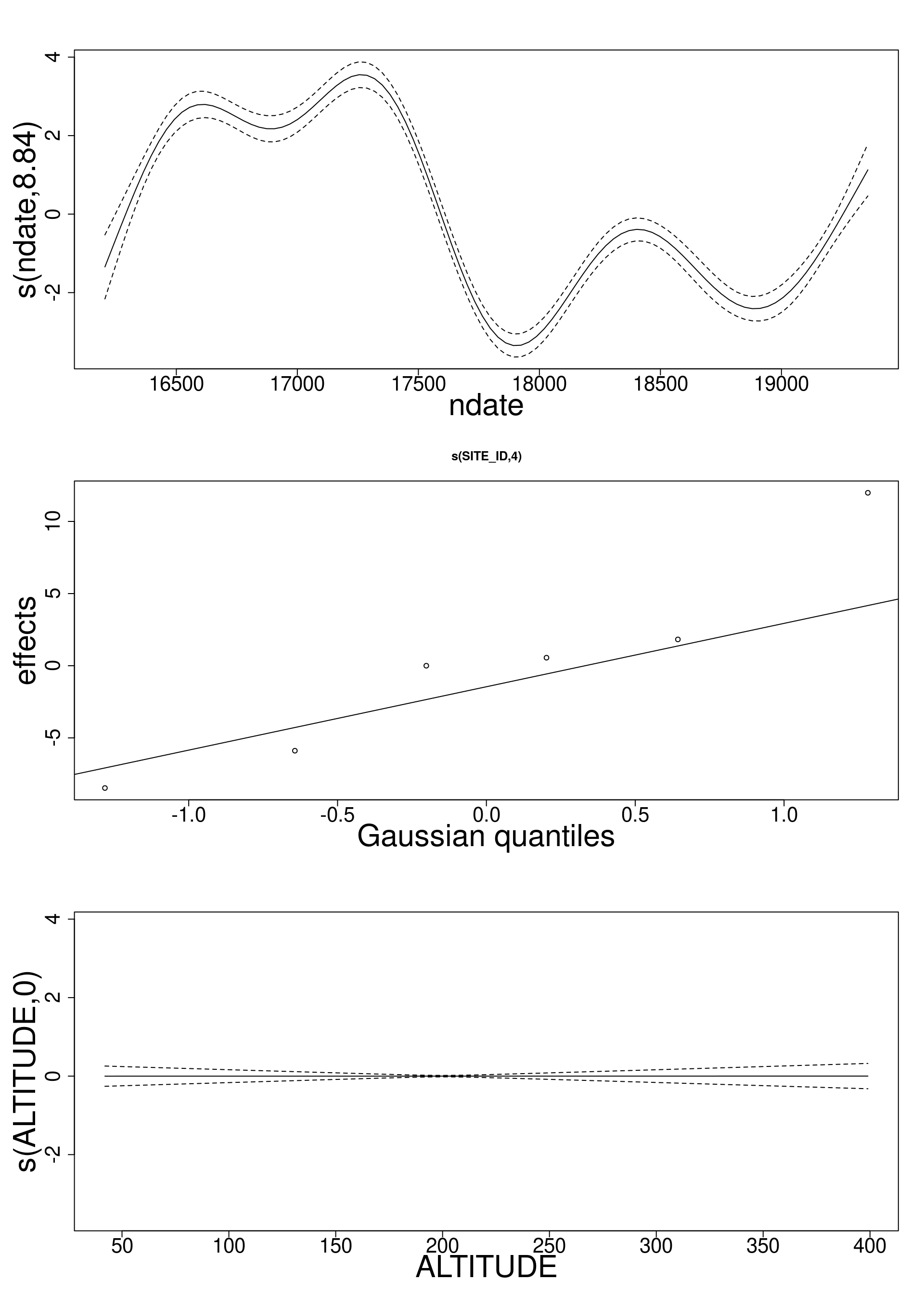
Where did we leave the analysis?
Where did we leave the analysis?
clear temporal variation from
s(ndate)clear between-site variation from
s(SITE_ID, bs= "re")- spatial variation not explained by
s(ALTITUDE, k= 5, bs= "ts")
- spatial variation not explained by
[...] Parametric coefficients:
Estimate Std. Error t value Pr(>|t|)
(Intercept) 39.821 3.550 11.216 <2e-16 ***
SOIL_TYPEOrganic soil 10.113 8.698 1.163 0.245
---
Approximate significance of smooth terms:
edf Ref.df F p-value
s(ndate) 8.8413793 8.992 165.574 <2e-16 ***
s(SITE_ID) 3.9983209 4.000 3777.345 <2e-16 ***
s(ALTITUDE) 0.0002275 4.000 0.008 0.637
--- - Is there a seasonal pattern?
- Is there any spatial trend?
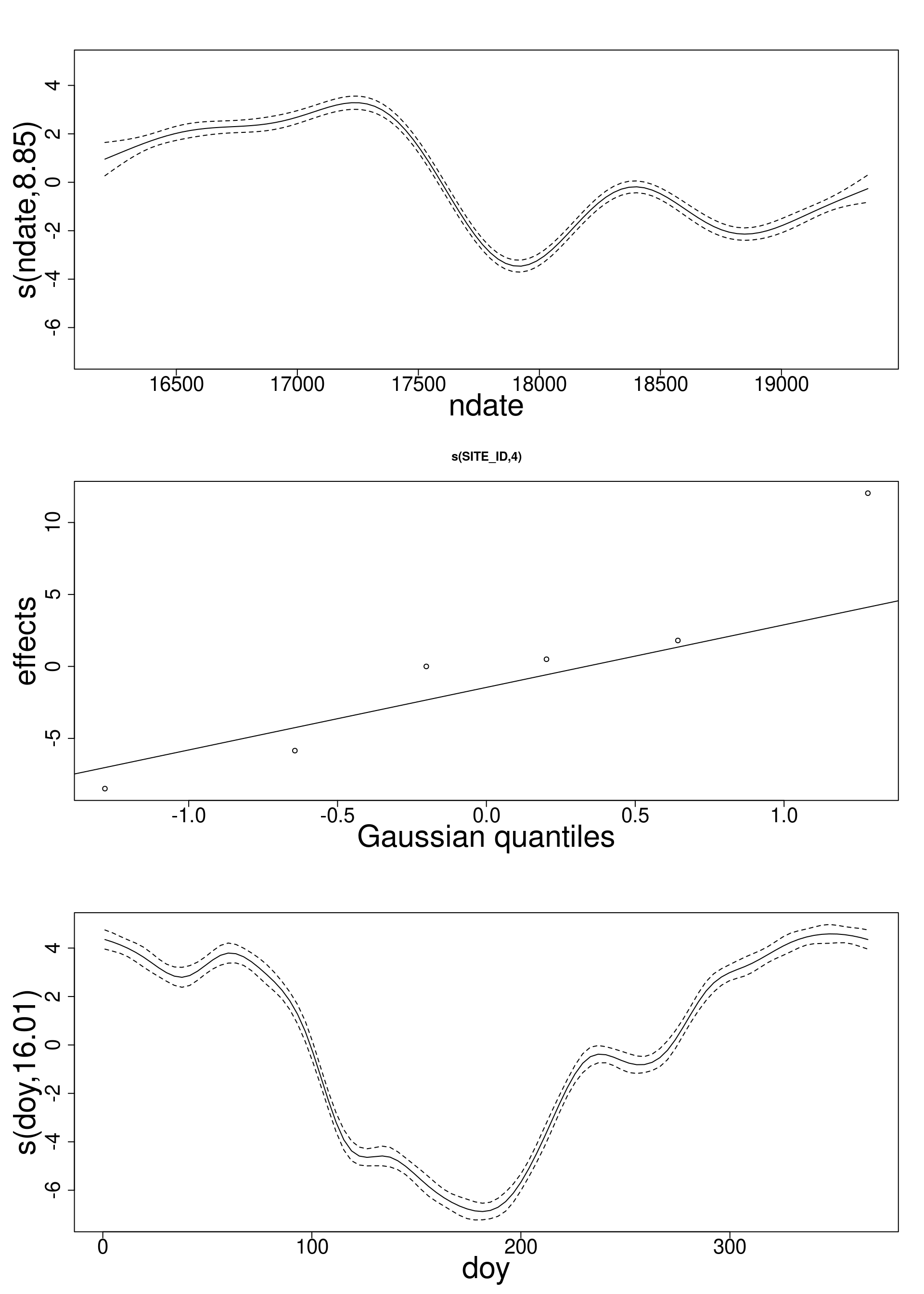
1. Is there a seasonal pattern?
Is there a seasonal pattern?
- = Repeatable pattern year-on-year
- Soil moisture on 31st December and on 1st Jan should be similar (ends should match):
- value
- curvature (up to 2nd derivative)
- Answer is a cyclic spline:
s(doy, bs= "cc")
Is there a seasonal pattern?
- = Repeatable pattern year-on-year
- Soil moisture on 31st December and on 1st Jan should be similar (ends should match):
- value
- curvature (up to 2nd derivative)
- Answer is a cyclic spline:
s(doy, bs= "cc")
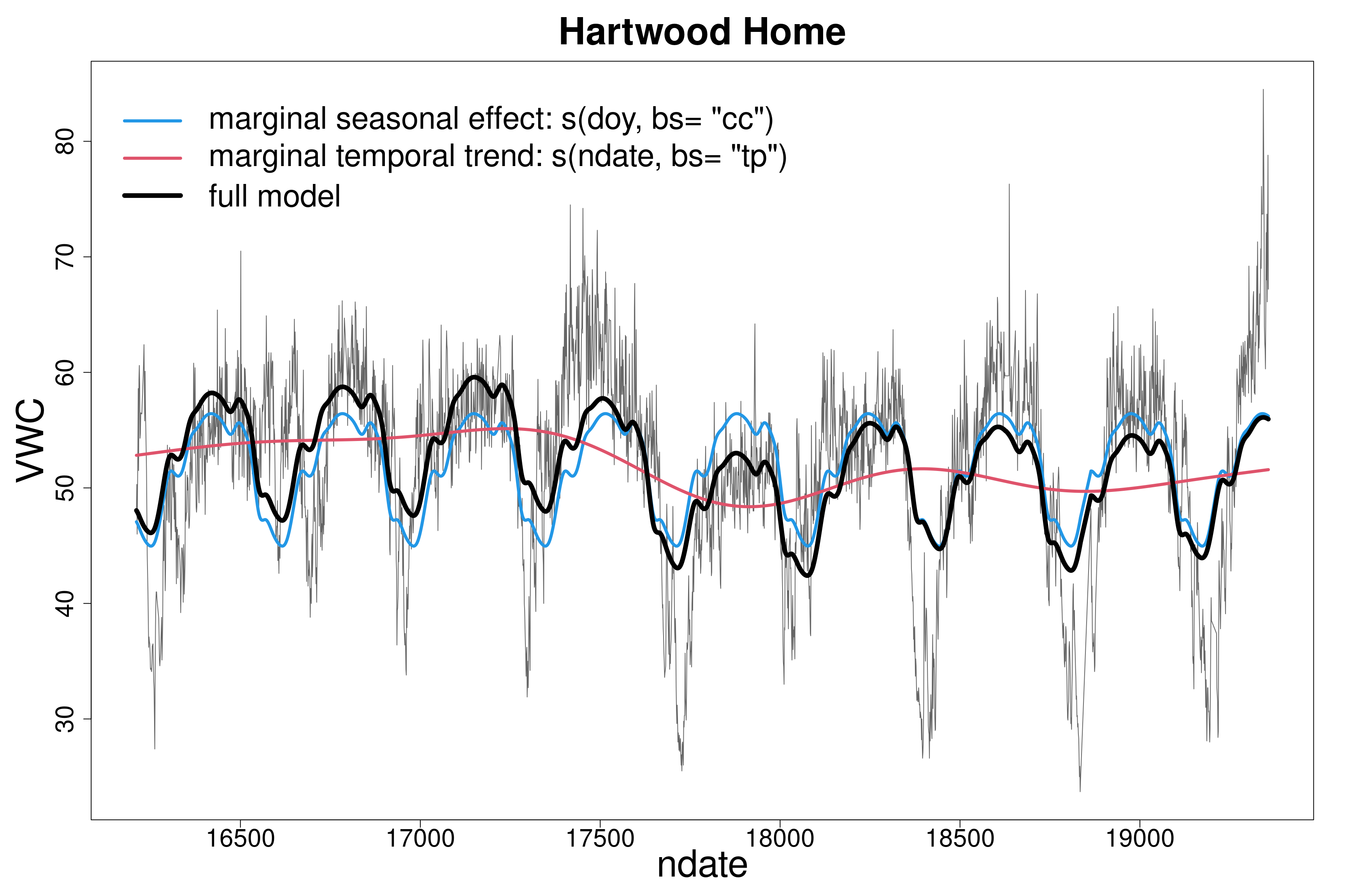
Is there a seasonal pattern?
Yes.
(together with a less structured temporal trend)
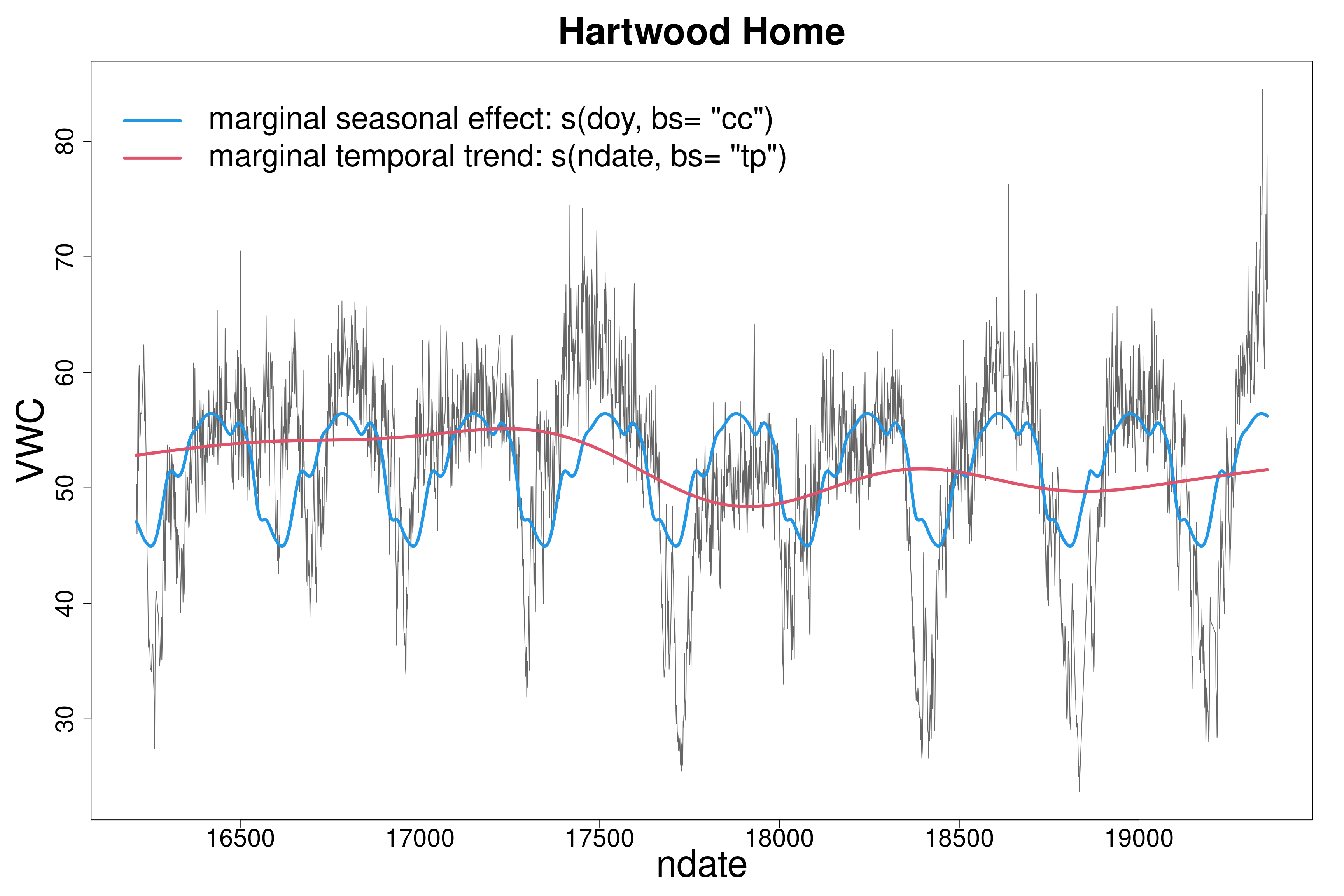
Is there a seasonal pattern?
Yes.
(together with a less structured temporal trend)
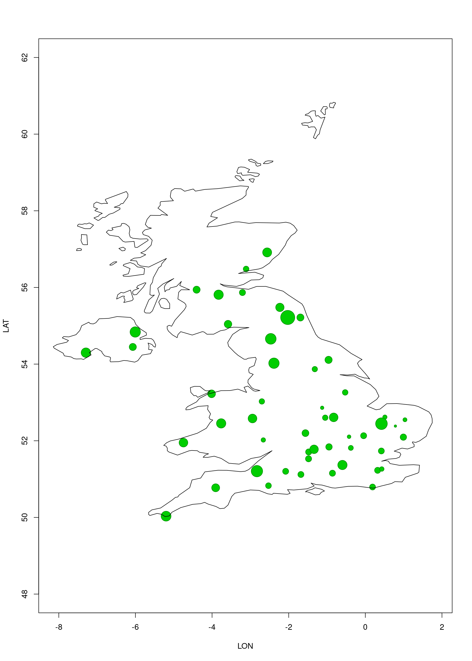
2. Is there any spatial trend?
Is there a general spatial trend?
Is there a general spatial trend?
- sounds like a smooth 2D surface…
- so, a bivariate (2D) spline?
- something like:
s(LON, LAT)
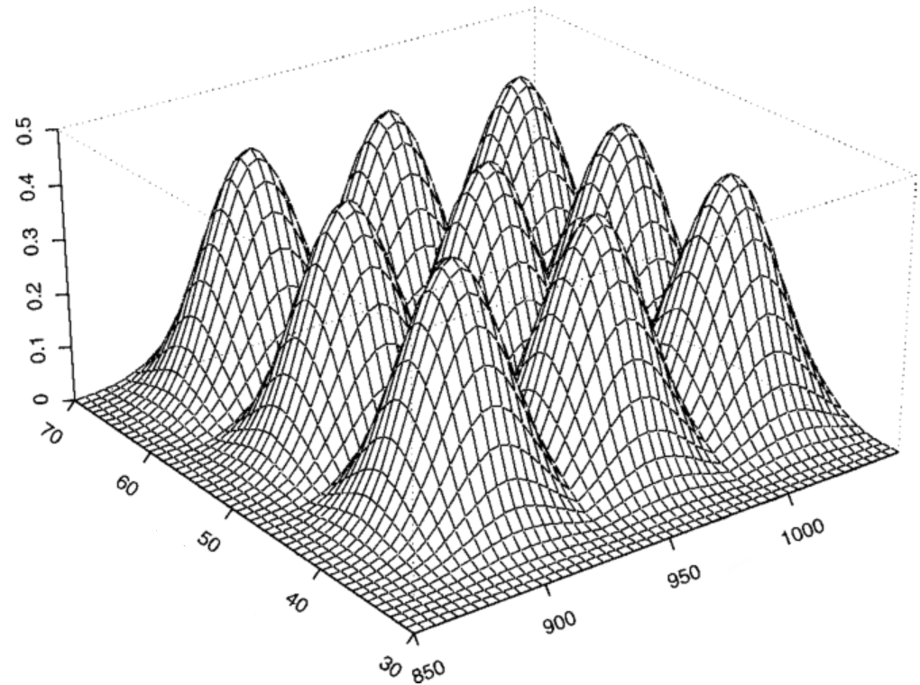
2D spline
- One way to do this:
- construct 2D spline bases (“volumes”)
- add them up with weights-> smooth surface
\[ s(X1,X2) = \sum_i \delta_{i} d_i(X1,X2) \]
- in mgcv,
s(X1, X2, k= n) - Generalizes to any number of dimensions
Intuition with 9 spline bases (k= 9)
Is there a general spatial trend?
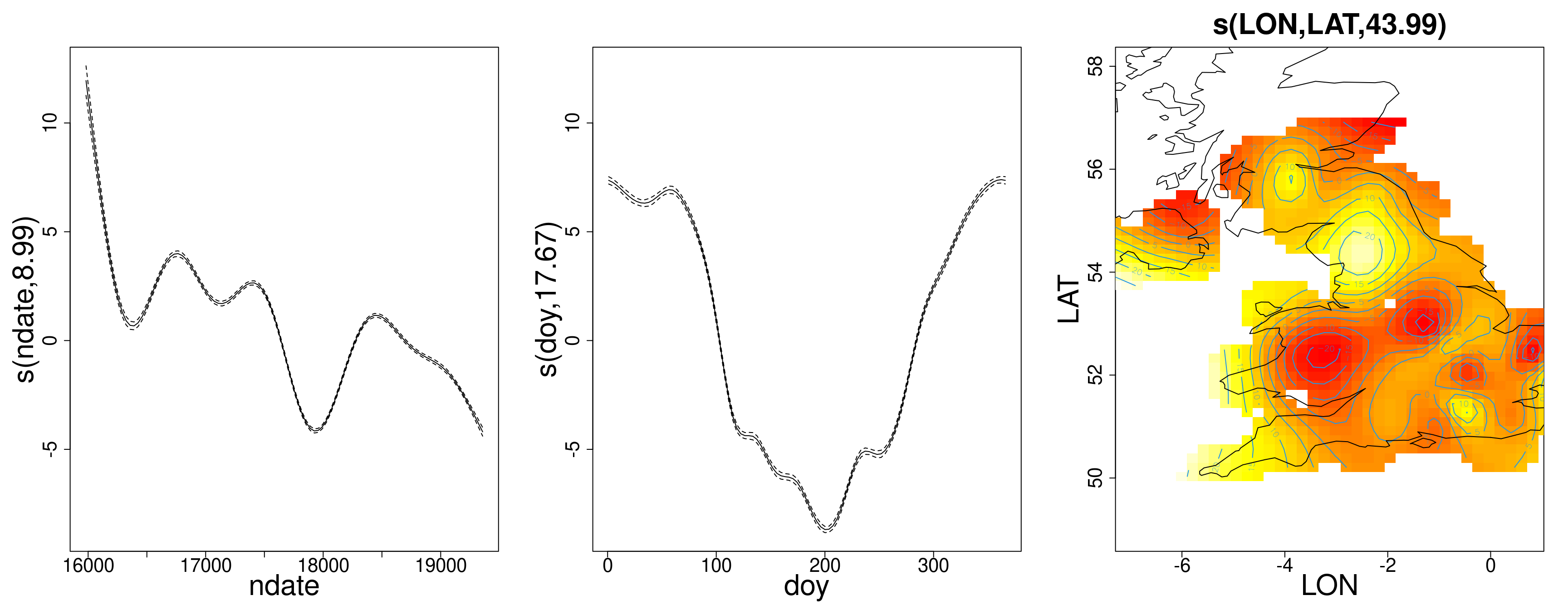
Was dropping the site random effect a good idea?
[...] Approximate significance of smooth terms:
edf Ref.df F p-value
s(ndate) 8.994 9 1714 <2e-16 ***
s(doy) 17.675 18 5452 <2e-16 ***
s(LON,LAT) 43.988 44 6655 <2e-16 ***
---
R-sq.(adj) = 0.826 Deviance explained = 82.6%
-REML = 4.1906e+05 Scale est. = 42.306 n = 127228
…………………………………………….(Probably not)
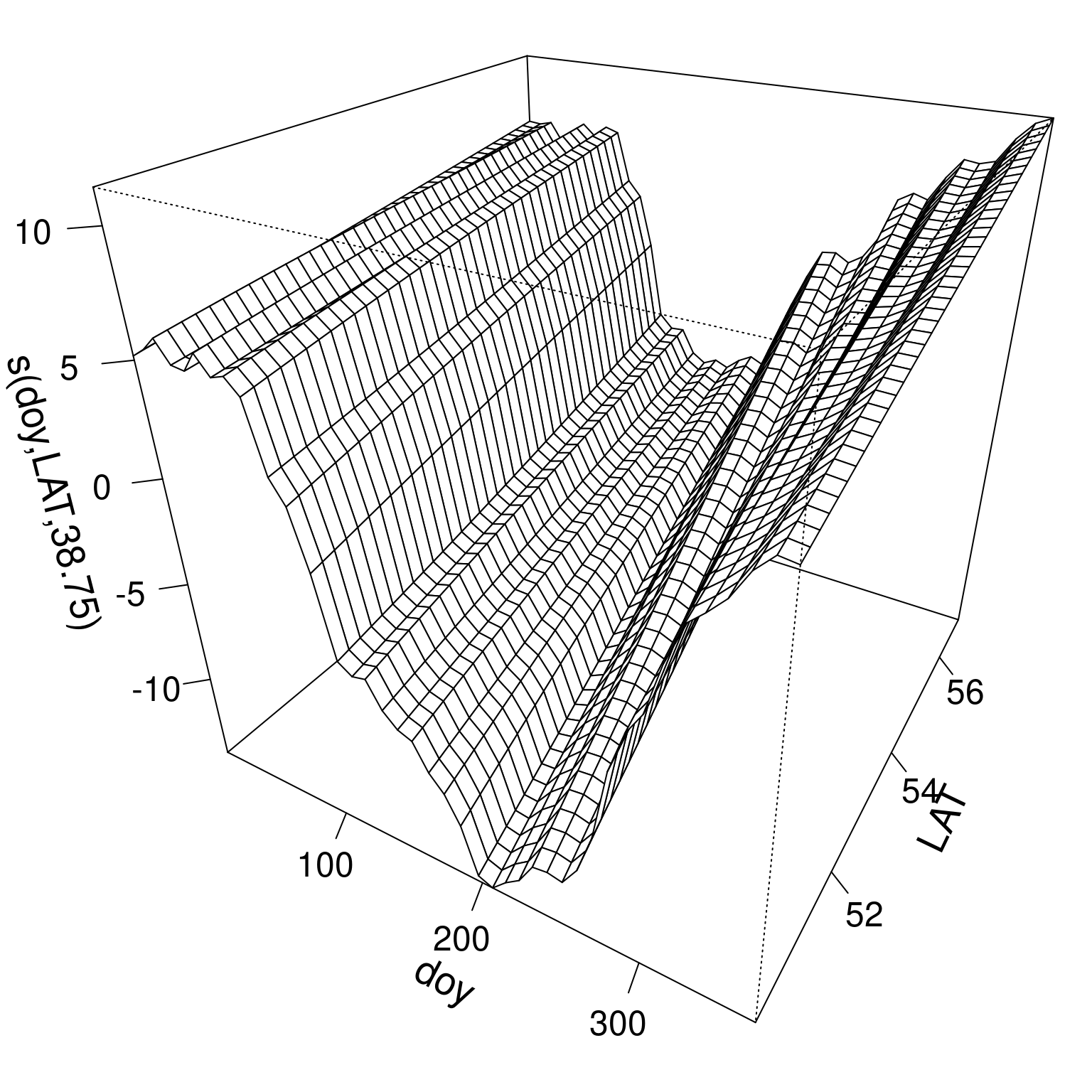
3. Does the seasonal pattern change with latitude? (space-time smoothing)
Space-time smoothing
Isotropy issue
LAT: 50 - 56° North (6 units range)doy: 1 - 366 days (365 units range)
Also,
- would like cyclic effect for
doy - but not for
LAT
Anisotropic multidimensional smoothing: tensor product smooths
Looking for a smooth function \(f(X1, X2)\)
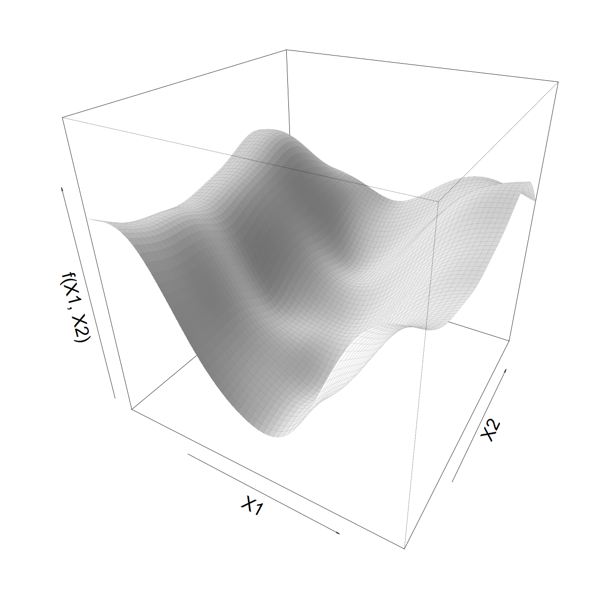
Smoothing over \(X1\)
- Let’s start with a standard 1D smoother
\[ s(X1) = \sum_k \beta_k b_k(X1) \]
- Built from basis functions \(b_k(X1)\)
- With coefficients \(\beta_k\) (“weights”)

Smoothing over \(X1\)
- Let’s start with a standard 1D smoother
\[ s(X1) = \sum_k \beta_k b_k(X1) \]
Built from basis functions \(b_k(X1)\)
With coefficients \(\beta_k\) (“weights”)
We want to let \(s(X1)\) vary with \(X2\)
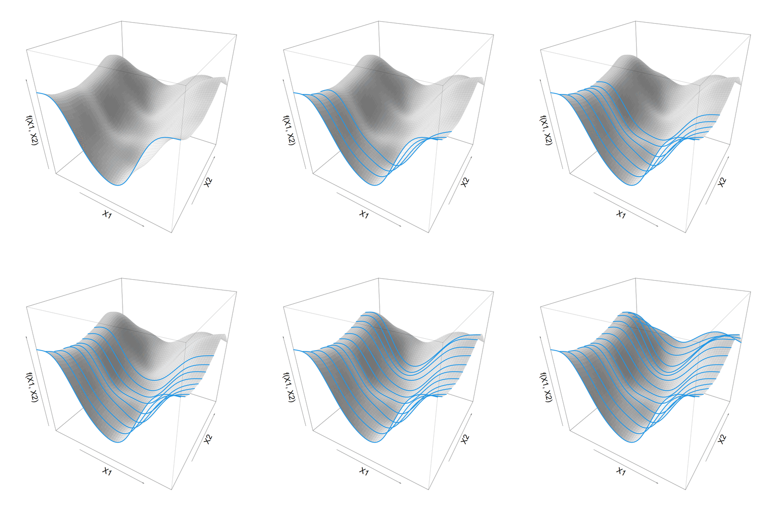
Making \(s(X1)\) vary smoothly with \(X2\)
- We have
\[ s(X1) = \sum_k \beta_k b_k(X1) \]
- Now, let \(s(X1)\) coefficients \(\beta_k\) be a 1D smooth function of \(X2\)
\[ \beta_k(X2) = \sum_j \alpha_{jk} a_j(X2) \]
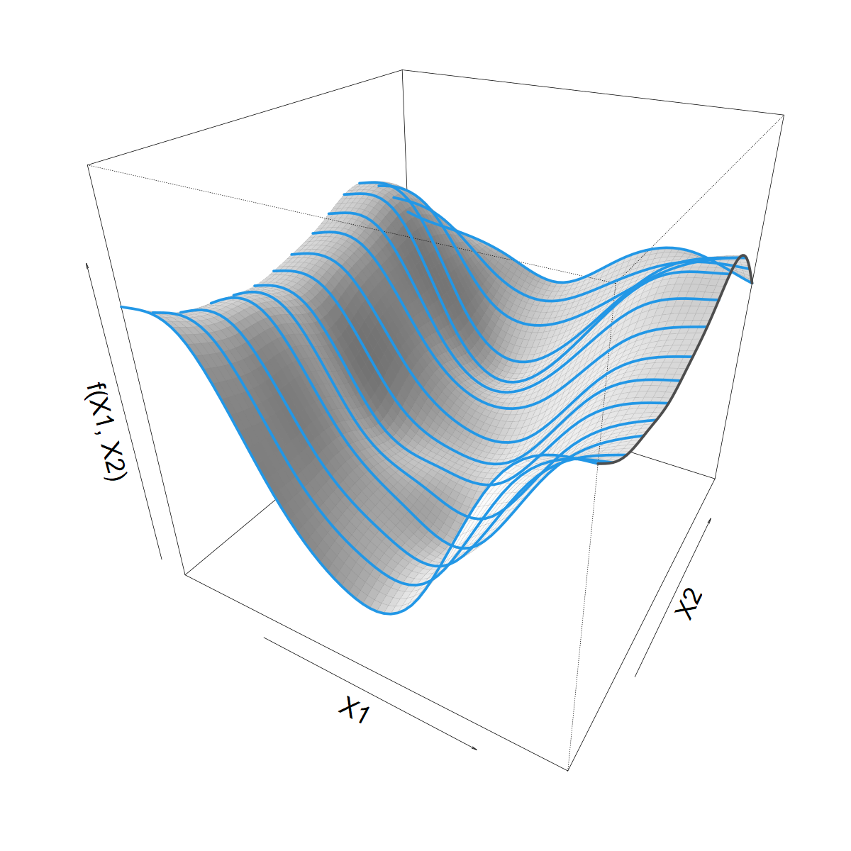
Making \(s(X1)\) vary smoothly with \(X2\)
\[ s(X1) = \sum_k \beta_k b_k(X1) \]
\[ \beta_k(X2) = \sum_j \alpha_{jk} a_j(X2) \]
Combining these 1D smooths gives a “tensor product”
\[ f(X1,X2) = \]
\[ \sum_j \sum_k \alpha_{jk} a_j(X2) b_k(X1) \]
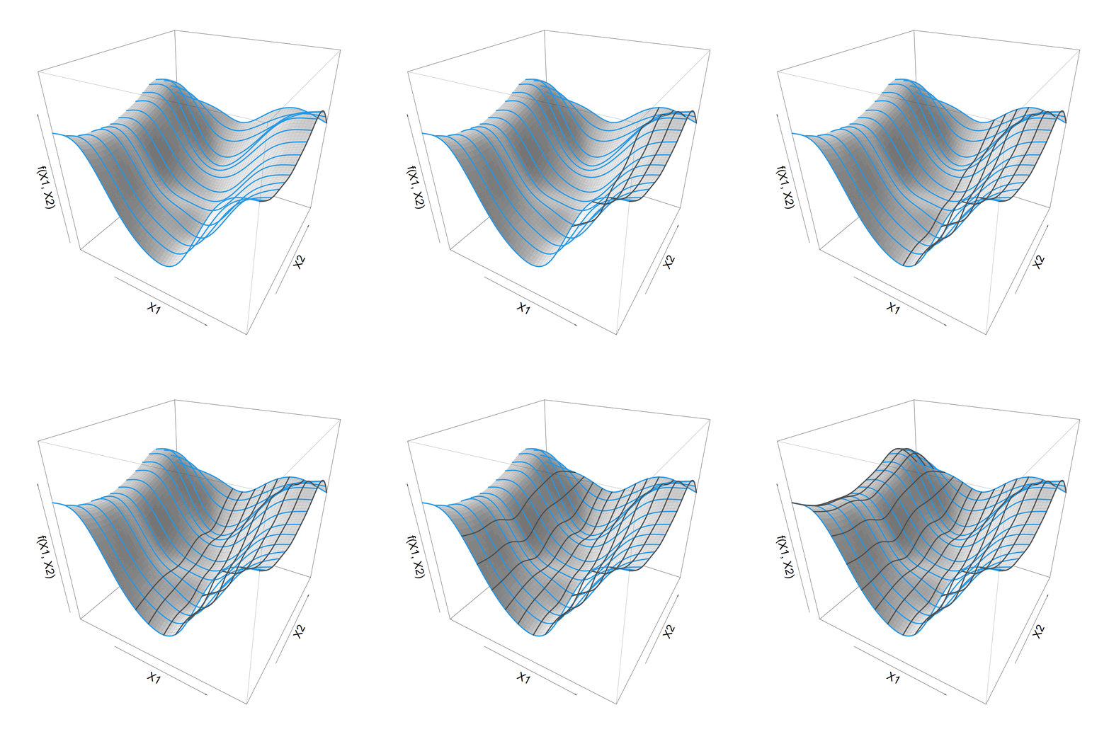
Isotropic vs. anisotropic smooth
2D spline
\[ s(X1,X2) = \]
\[ \sum_i \delta_{i} d_i(X1,X2) \]

- Single multivariate spline
- Same smoothness in all directions
Tensor product
\[ f(X1,X2) = \]
\[ \sum_j \sum_k \alpha_{jk} a_j(X2) b_k(X1) \]

- Product of 1D splines per margin
- Different spline types & penalties
Isotropic vs. anisotropic smooth
2D spline

In mgcv,
s(X1,X2, k=n, bs="tp")
Tensor product

In mgcv,
te(X1,X2, k=c(n1,n2), bs=c("tp","cc"))
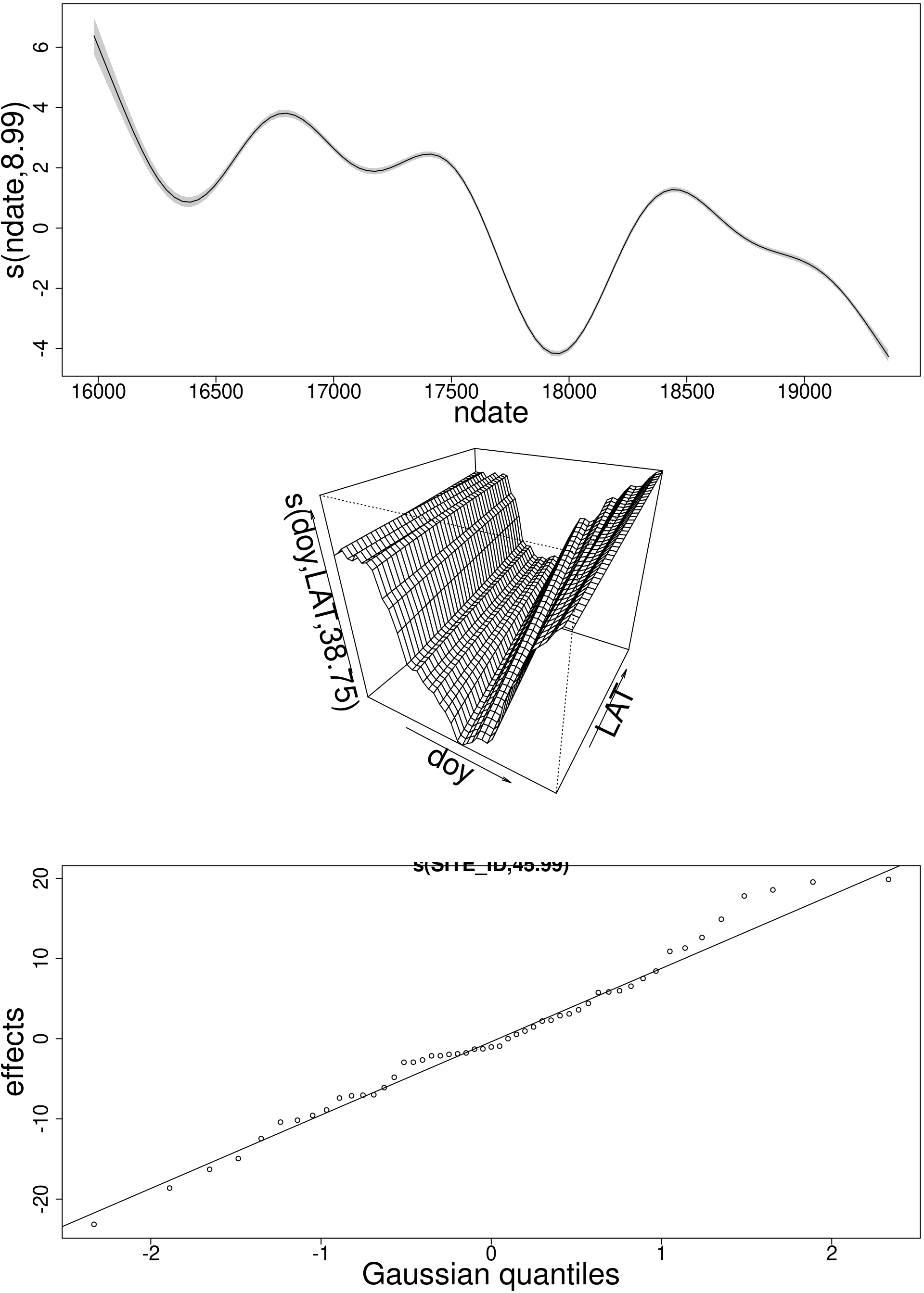
Space-time smoothing in practice
te(doy, LAT, bs= c("cc", "tp"))

Interpreting the space-time smooth
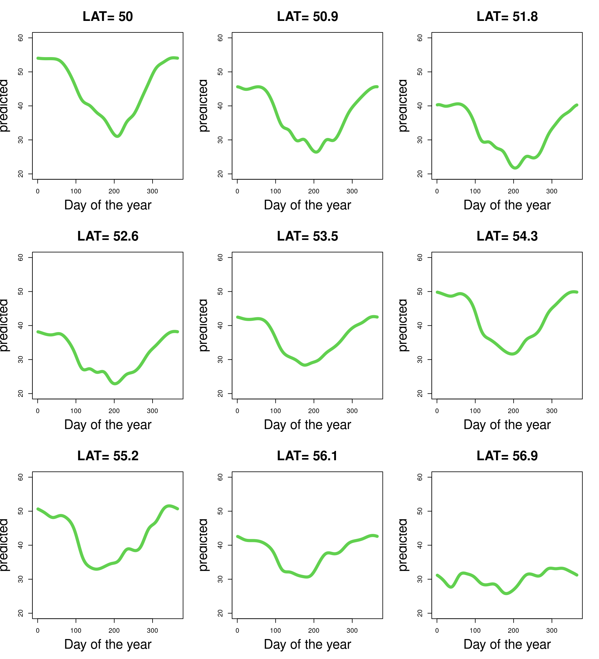
Predicting for a range of set latitudes
LAT_vec<- seq(min(all_sites$LAT),
                max(all_sites$LAT), l= 9)

par(mfrow= c(3, 3))
for(i in 1:9){
  predicted<- predict(b_seaslat,
     newdata= data.frame(
       all_sites[1, c("SOIL_TYPE",
                        "ndate",
                        "SITE_ID")],
       doy= 1:365,
       LAT= LAT_vec[i]
     )
  )

  plot(1:365, predicted, type= "l",
        xlab= "Day of the year",
        main= paste("LAT=", round(LAT_vec[i], 1)),
        ylim= c(20, 60))
}
Limitations
- CI too narrow
- Overfitting
- WHY?
- non-independence
- heterogeneity of variance?
- bias / lack of fit?
- …
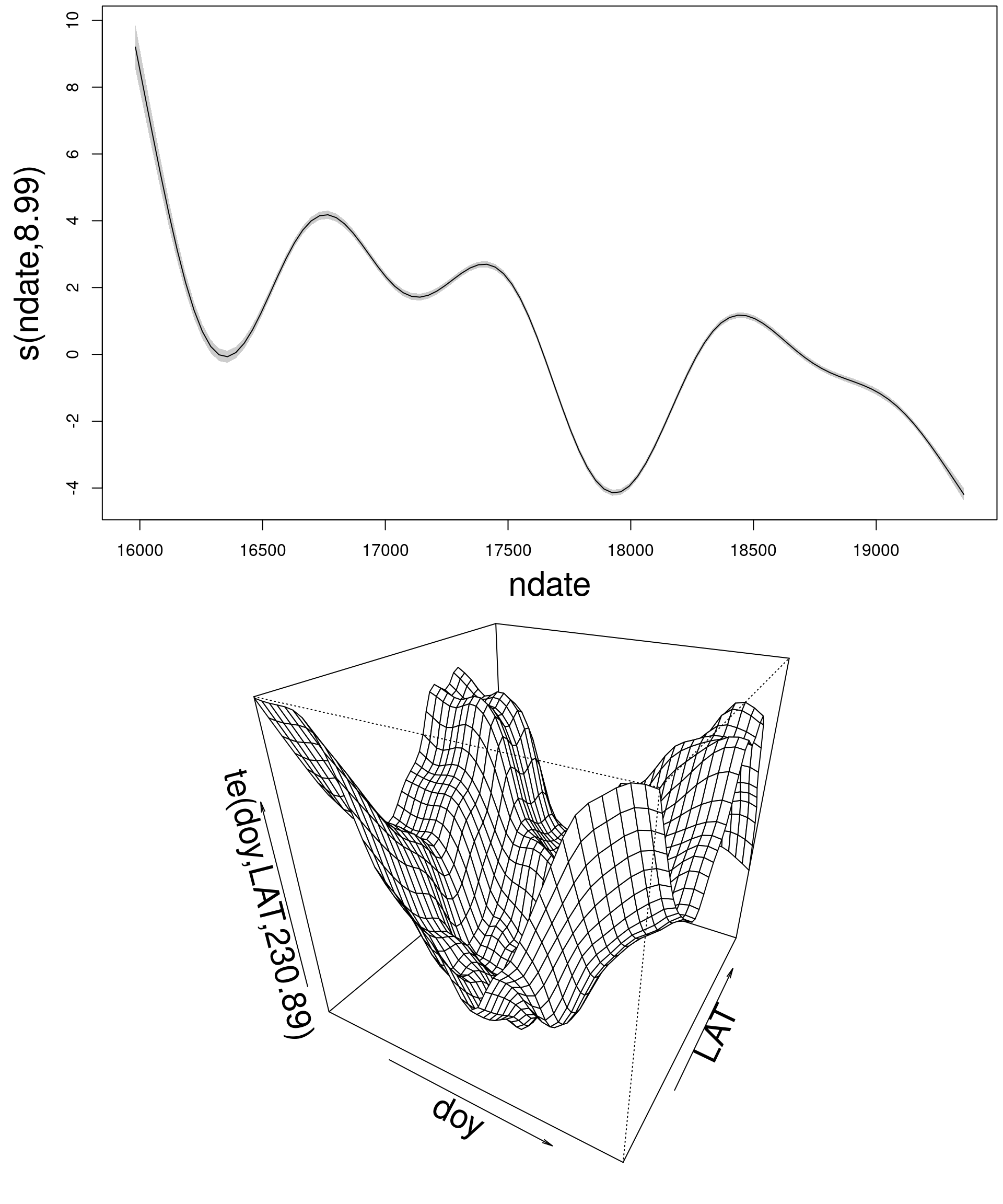
Overfitting: curse or blessing?
- GAMs particularly sensitive to assumptions
- non-independence
- variance heterogeneity
- Leads to overfitting (too much wigglyness)
- Overfitting less apparent in simpler LM / GLMs
- confidence limits too narrow
- model selection favoring too large models
- Overfitting → model diagnostic opportunity
- Need domain expertise and critical evaluation
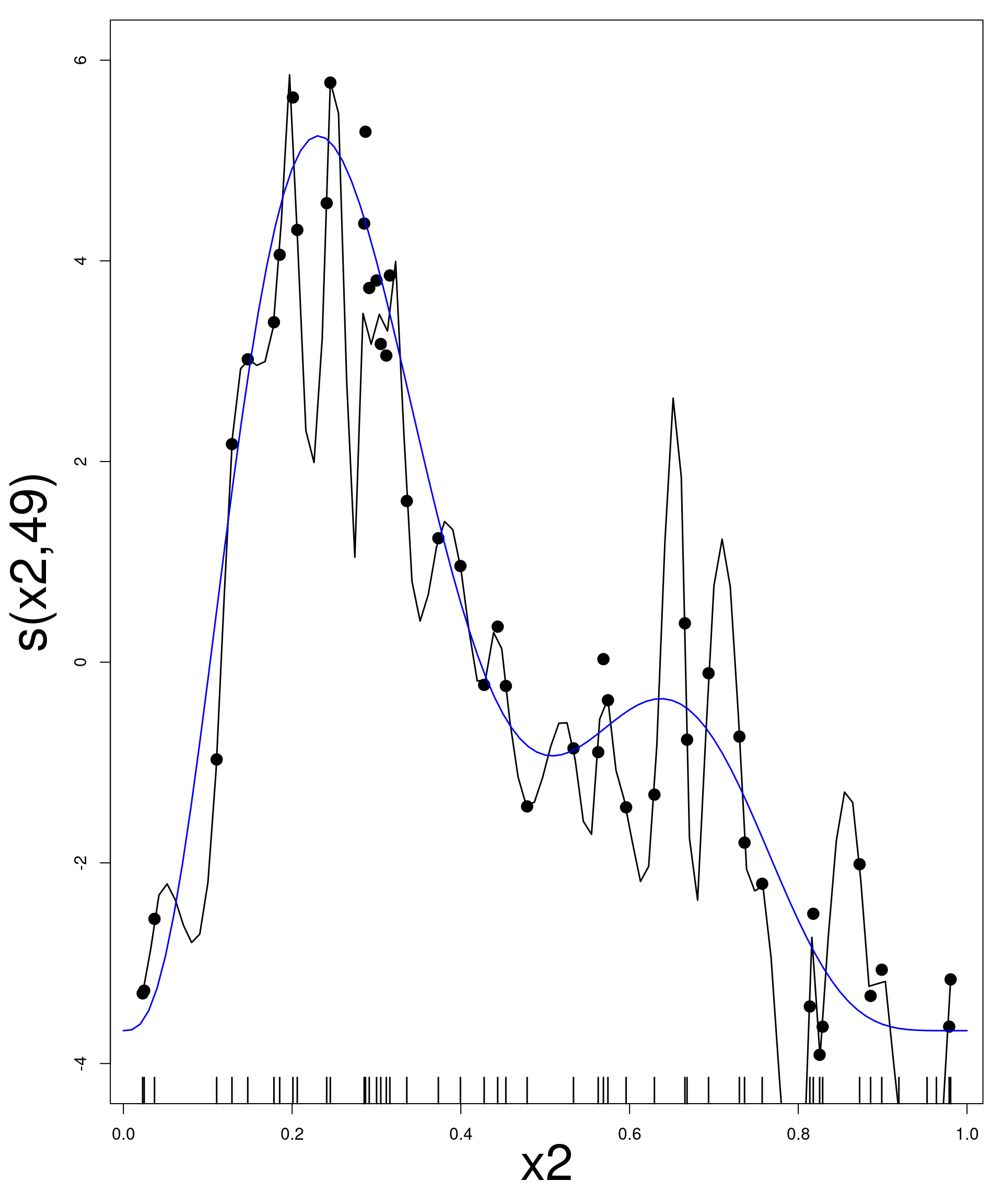
More advanced GAMs
- Mixed-effect GAMs: non-independence by space, time, cluster, etc…
- Hierarchical GAMs (random curves)
- Univariate / multivariate Likelihoods
- Many more spline types available
- GAMs for big data sets:
bam(used mostly likegam) - Functional modelling
Cumulative effect of rainfall on soil wetness
- Wetness affected by rainfall
- Not just on the day
- Cumulative effect of previous days (lags)

gam(VWC ~ SOIL_TYPE + R0 + R1 + R2 + R3 + R4 + R5 + R6 + R7 + s(SITE_ID, bs= "re"))could be problematic- Possible interactions between lags, e.g.
- hydrophobicity due to draught
- soil saturation after heavy rain
- Functional regression to the rescue
f(Rainfall, Lag)
Recap
- Ad-hoc cyclic patterns:
bs= "cc" - Multivariate smooths
- isotropic
s(X1,X2) - anisotropic
te(X1,X2)
- isotropic
- Interpretation in 3D or more:
- slicing the salami (haggis) can help
- decomposing the smooth (optional exercise)
- Check model carefully. Where’s Wiggly? 👀

Image credits
MarxEilers.png from B. D. Marx and P. H. C. Eilers, “Multidimensional Penalized Signal Regression,” Technometrics, vol. 47, no. 1, pp. 13–22, Feb. 2005, doi: 10.1198/004017004000000626.
balloons_cappadocia.jpg by Alexey Komarov (CC BY 2.0 Deed)
tennis-product-smoosh.png by T.Cornulier (CC BY 4.0 Deed)
spine.jpg by M.Baird (CC BY 2.0 Deed)
leek.jpg by Joy (CC BY 2.0 Deed)
WheresWallyCrop.jpg modified from W.Murphy (CC BY-SA 2.0 Deed)

