library(mgcv)
load("cosmos-processed.RData")

wwoods <- subset(all_sites, SITE_NAME=="Wytham Woods")

b <- gam(COSMOS_VWC ~ s(ndate, k=20), data=wwoods, method="REML")

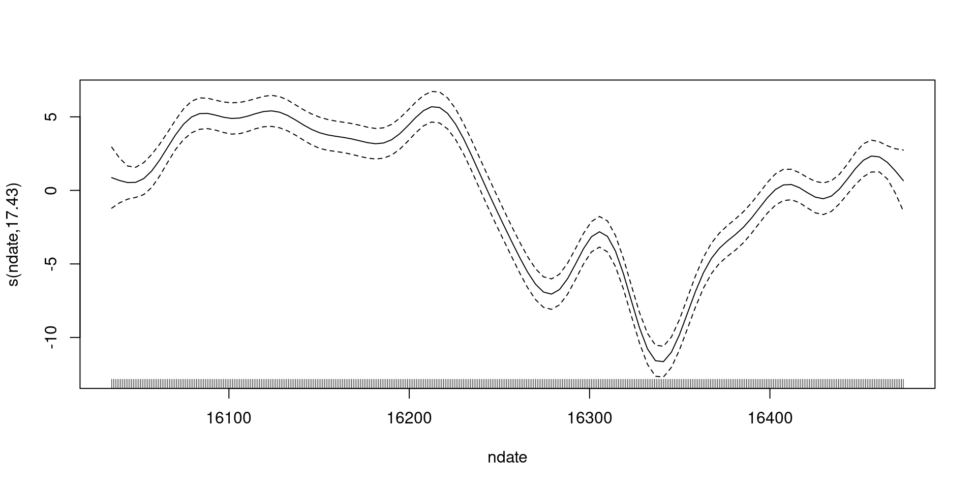
plot(b)Predictions and variance
David L Miller
Biomathematics and Statistics Scotland
UK Centre for Ecology and Hydrology
What can we do?
- Use
gam()to fit a model - Use
summary()to assess it - Use
plot()to visualise it
Going back to our model

Now we can fit a model,
now we are dangerous
What do we want to do with our model?
- For linear models, we often interpret coefficients
- We don’t have that here
- So we usually make predictions and plots
(Intercept)  s(ndate).1  s(ndate).2  s(ndate).3  s(ndate).4  s(ndate).5
 47.3525000   7.5801107  13.8527308  -4.1595358 -12.1449614  -3.0512930
 s(ndate).6  s(ndate).7  s(ndate).8  s(ndate).9 s(ndate).10 s(ndate).11
 -8.8018184   0.8292287  -6.1265129  -7.6962263  12.2316442   7.0850161
s(ndate).12 s(ndate).13 s(ndate).14 s(ndate).15 s(ndate).16 s(ndate).17
 -5.2282569   3.6549750  -0.2188604  -0.3257381   9.7677258   7.0620897
s(ndate).18 s(ndate).19
 18.6422253 -12.5062881
Wait, what are we seeing in that plot?

What do we have?
- The black line:
s(nday)- (what about \(\beta_0\)?)
- Dashed line:
s(nday)\(\pm 2\) standard errors- (how do we get to that?)
- (what uncertainty is included?)
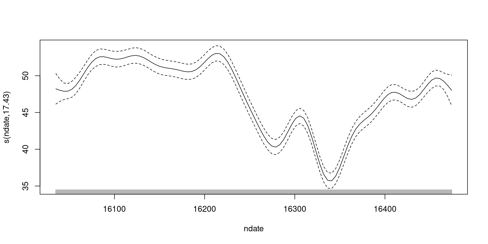
shifting to include the intercept

Including uncertainty in the intercept

How do we make these plots?
- Black line is a prediction
- \(\beta_0 + s(t)\) over values of \(t\)
How do we make these plots?
- Black line is a prediction
- \(\beta_0 + s(t)\) over values of \(t\)
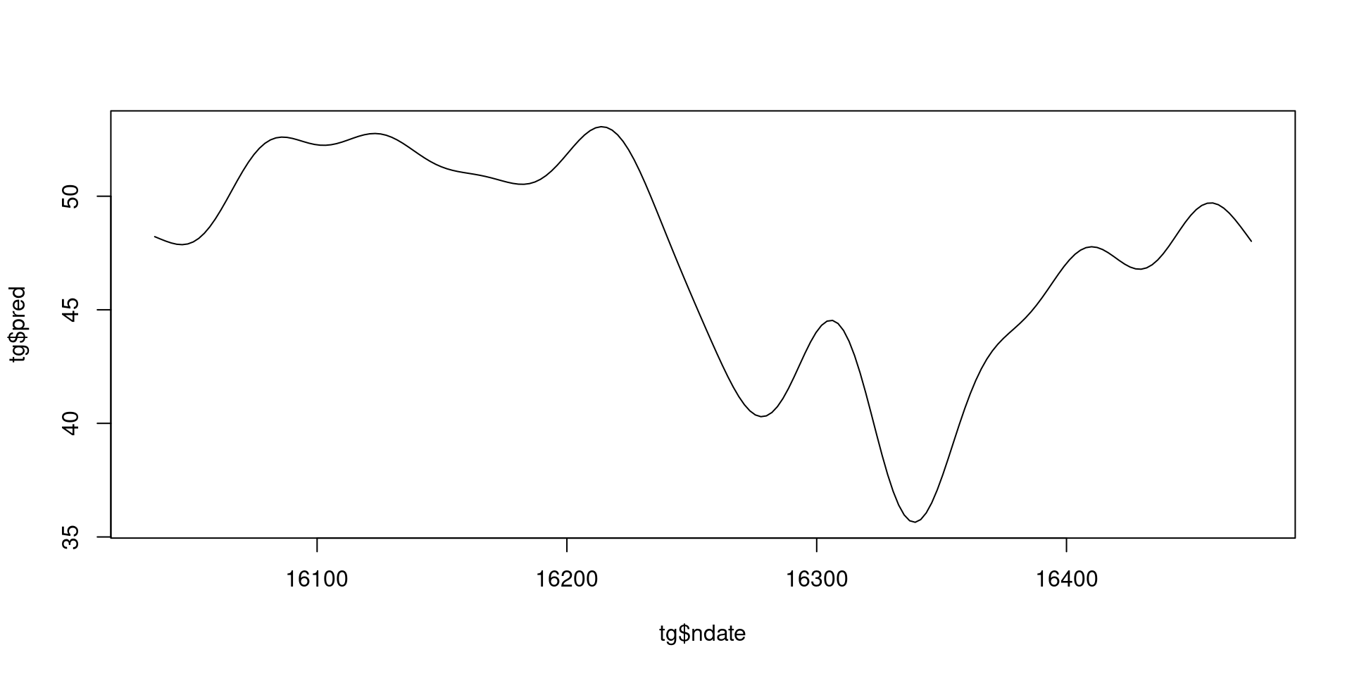
Recipe:
- Make a grid
- Use
predict()to make predictions over the grid
Doing that in R
Doing that in R (extra bits)
- Note that our
newdata=needs to have all the covariates in it - Calling
predict(b)just gives us fitted values
And we can plot that…

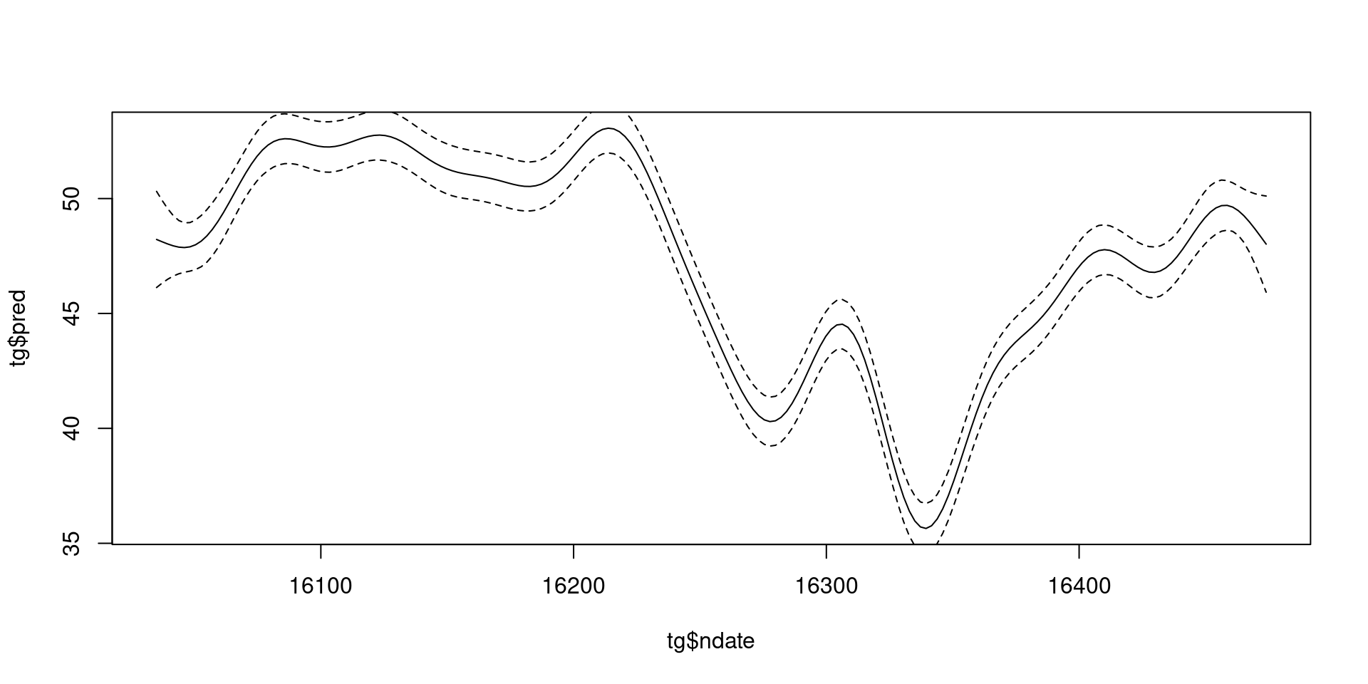
What about uncertainty?
predict(..., se=TRUE) gives standard errors
List of 2
 $ fit   : num [1:200(1d)] 48.2 48.1 48 47.9 47.9 ...
  ..- attr(*, "dimnames")=List of 1
  .. ..$ : chr [1:200] "1" "2" "3" "4" ...
 $ se.fit: num [1:200(1d)] 1.046 0.899 0.767 0.657 0.579 ...
  ..- attr(*, "dimnames")=List of 1
  .. ..$ : chr [1:200] "1" "2" "3" "4" ...
Building that plot

What do these intervals mean?
- These are really credible intervals
- … but they have good 🎲frequentist🎲 properties
- (so we can call them confidence intervals)
- What do they say?
- they are “across-the-function” intervals
- thinking about if \(s(x) = 0 \quad \forall x\)
- (a bit more complicated becuase of centering)
- see
summary()
Thinking about intervals…
- Why are they credible intervals?
- Because we can think of the penalty as a prior
- Then we have a posterior for our model
- … and we can do 🔮posterior sampling🔮
- (more on that in a minute)
Where did that uncertainty come from?
- So far we’re only looking at uncertainty from \(\hat{\boldsymbol{\beta}}\)
- What about smoothing paramter (\(\lambda\)) uncertainty?
- We estimate a parameter, we need some uncertainty!
- For
predict()andplot()we can useunconditional=TRUE- (doesn’t make a difference for this data)
Posterior sampling

Posterior sampling background
From ⚡theory⚡ \(\boldsymbol{\beta} \sim \text{MVN}(\hat{\boldsymbol{\beta}}, \Sigma)\)
So, we can 🔮simulate🔮 from that distribution
Make lots of predictions
- make a prediction matrix and multiply by the simulated parameters
This generalizes very well, so we can make predictions of more than just smooths
Miller et al (2022) and Miller (2021) have more details
More on predict()
- We’ll use more features of
predict()later type=argument changes the type of prediction- By default on the link scale (fine here for normal)
"response"to put on the response scale"iterms"to give per term predictions"lpmatrix"for a prediction matrix- Don’t worry about this for now!
Recap
plotshows us basic plots- we can make them ourselves if we want!
- Make predictions using
predict()- Need to fiddle to make the data
- Use
se.fit=TRUEto get uncertaintyunconditional=TRUEgive us smoothing parameter uncertainty
- Uncertainty comes from smooth parameters and smoothing parameters
- Intervals can be used to check if the smooth is zero