What are GAMs?

David L Miller

Biomathematics and Statistics Scotland

UK Centre for Ecology and Hydrology

Overview

• A very quick refresher on GLMs
• What is a GAM?
• How do GAMs work? (Roughly)
• What is smoothing?
• Fitting and plotting simple models

First…

A (very fast) refresher on (G)LMs

First, linear models

• Models that look like:

\[ y_i \sim \text{Normal}(\mu_i, \sigma_i) \]

• where:

\[ \mu_i = \beta_0 + \beta_1 x_{1i} + \beta_2 x_{2i} + \ldots \]

• Roughly: want to make \(y_i\) with weighted bits of the \(x_{ji}\)s

What is a Generalized Linear model (GLM)?

• Models that look like:

\[ y_i \sim \text{EF}(\mu_i, \sigma_i) \]

• where:

\[ g(\mu_i) = \beta_0 + \beta_1 x_{1i} + \beta_2 x_{2i} + \ldots \]

• \(g\) is a link function
• \(\text{EF}\) is an exponential family distribution
  • Normal, Poisson, Binomial (all our usual friends)

What is a Generalized Linear model (GLM)?

• Models that look like:

\(y_i \sim \text{EF}(\mu_i, \sigma_i); \qquad g(\mu_i) = \beta_0 + \beta_1 x_{1i} + \beta_2 x_{2i} + \ldots\)

What does that mean?

The the response, \(\mu_i\), is assumed to be a linear combination (weighted by the \(\beta\)s) of the covariates, \(x_{ji}\), with an intercept (\(\beta_0\)).

Why bother with anything more complicated?

Is this linear?

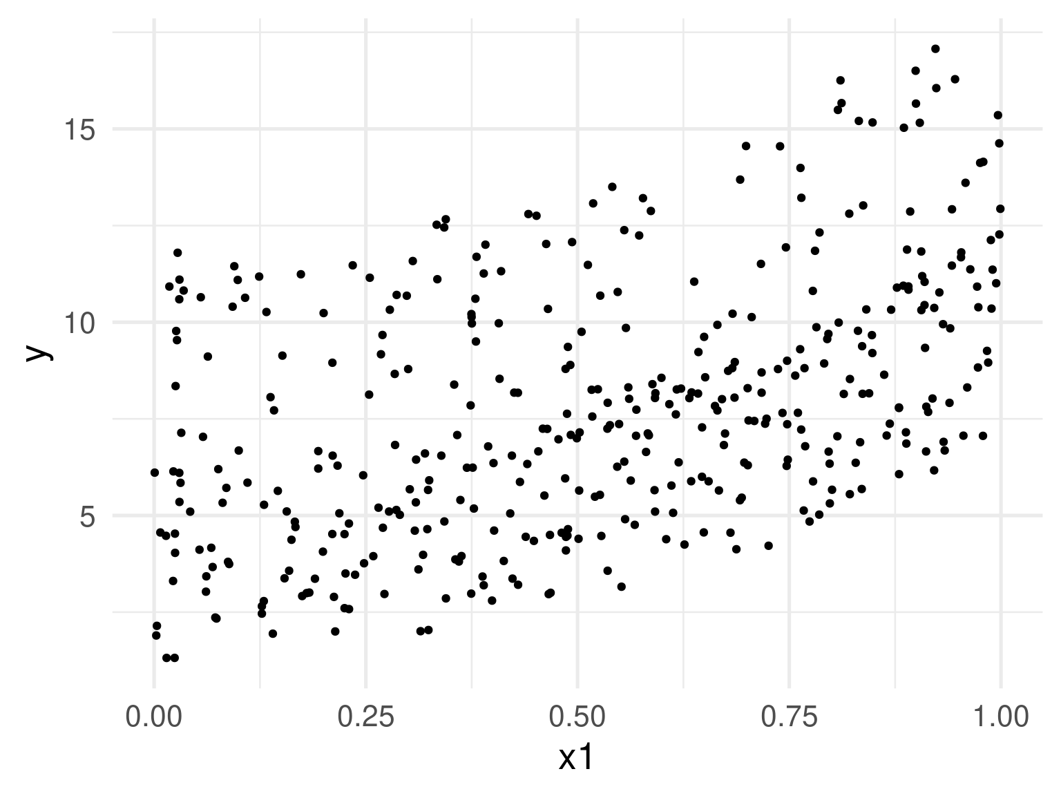
Is this linear? Maybe?

lm(y ~ x1, data=dat)

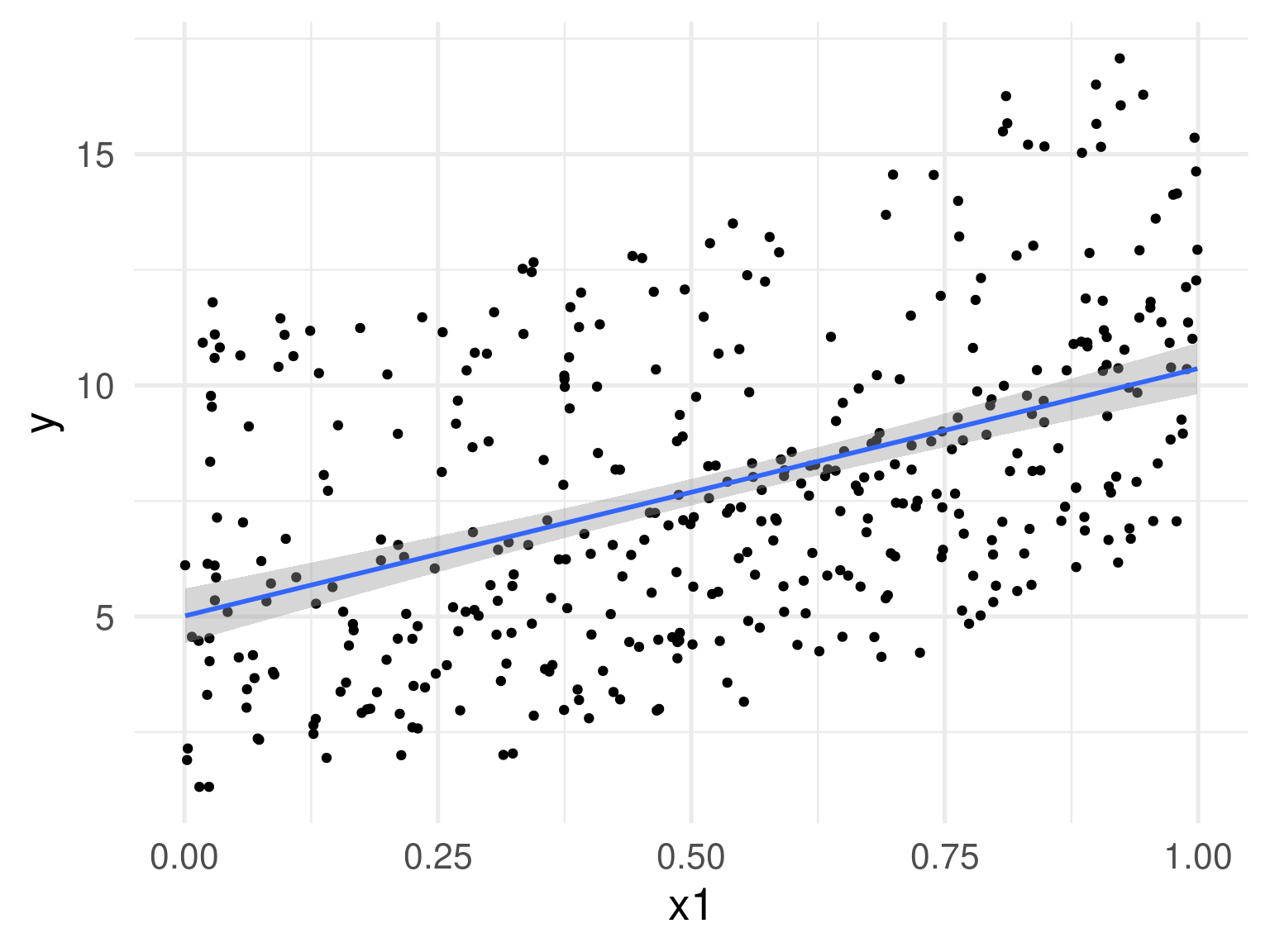
Is this linear? Maybe???

lm(y ~ poly(x1, 2), data=dat)

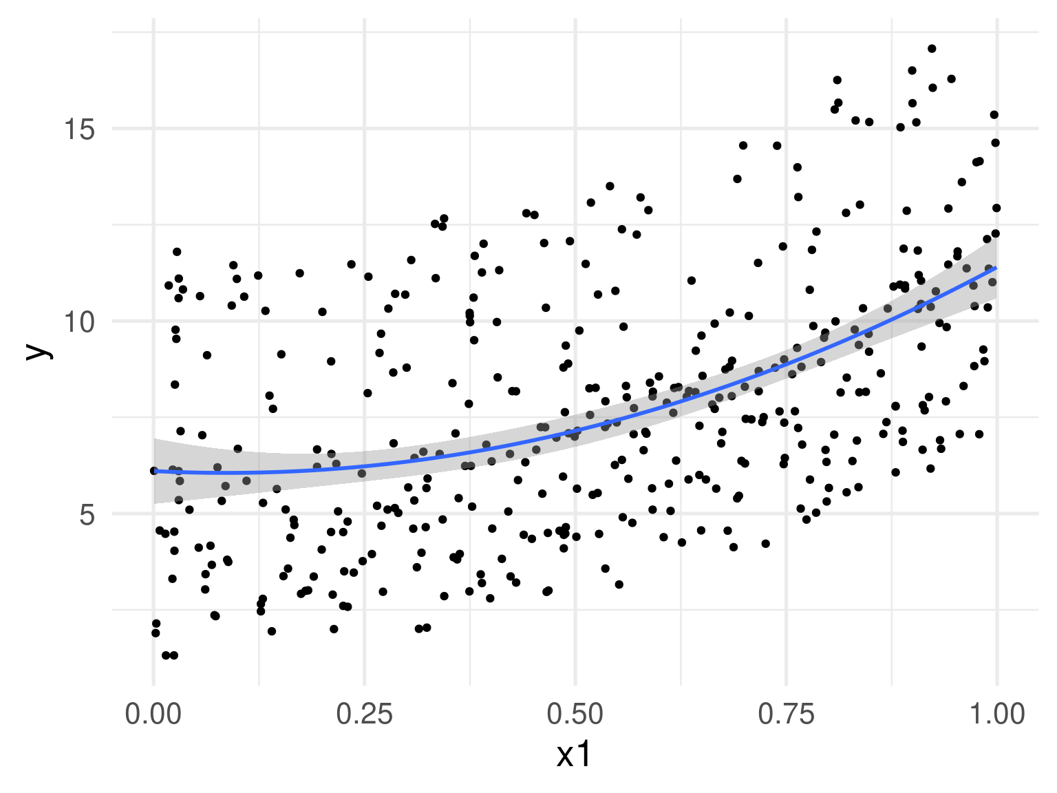
Is this linear? Maybe not.

lm(y ~ poly(x1, 2), data=dat)

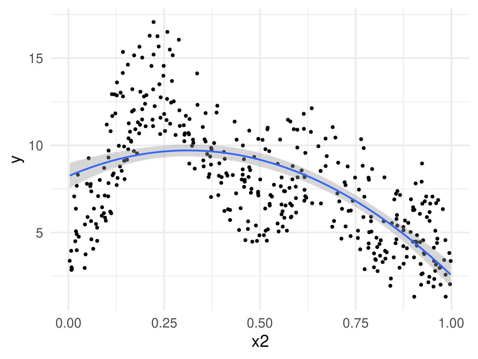
Can we keep adding polynomial terms?

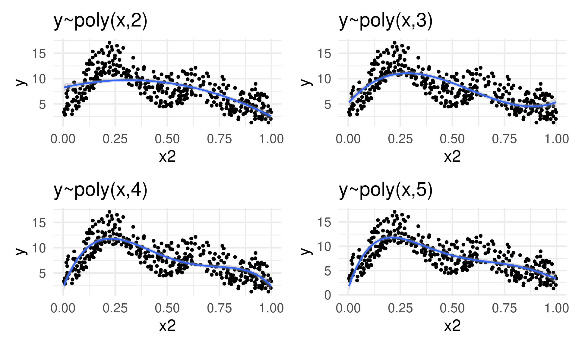
No

(for a few reasons)

Polynomial terms aren’t the answer

• No control of overfitting
• Computationally difficult to deal with (esp. with higher orders)

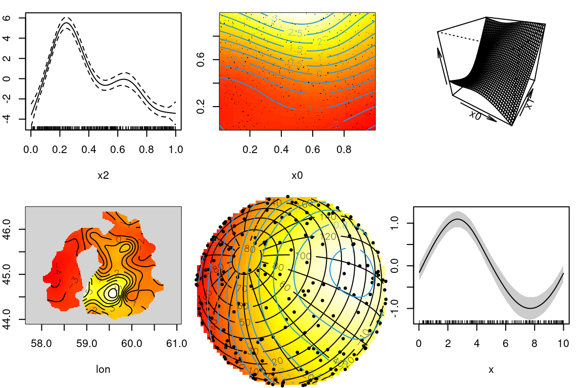
If we want to add wiggly effects, we use a GAM

Requirements

• Control for overfitting
• Flexible
• Fit within a framework we know

GAM examples

How do we make wiggly functions?

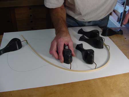
Splines (historical)

Splines (historical)

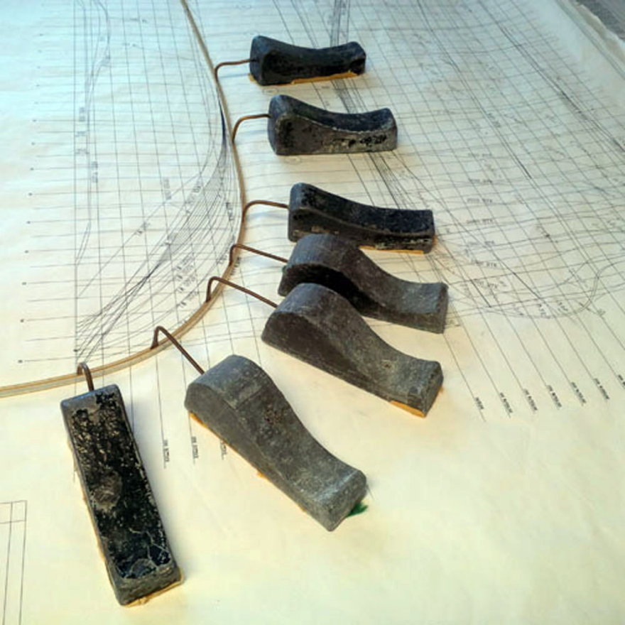
Photos from https://www.core77.com/posts/55368/When-Splines-Were-Physical-Objects

Smoothers

• Make flexible functions from adding simpler functions

\[ s(x) = \sum_k \beta_k b_k(x) \]

• Built from basis functions \(b_k(x)\)
• Only need to estimate \(\beta_k\)s

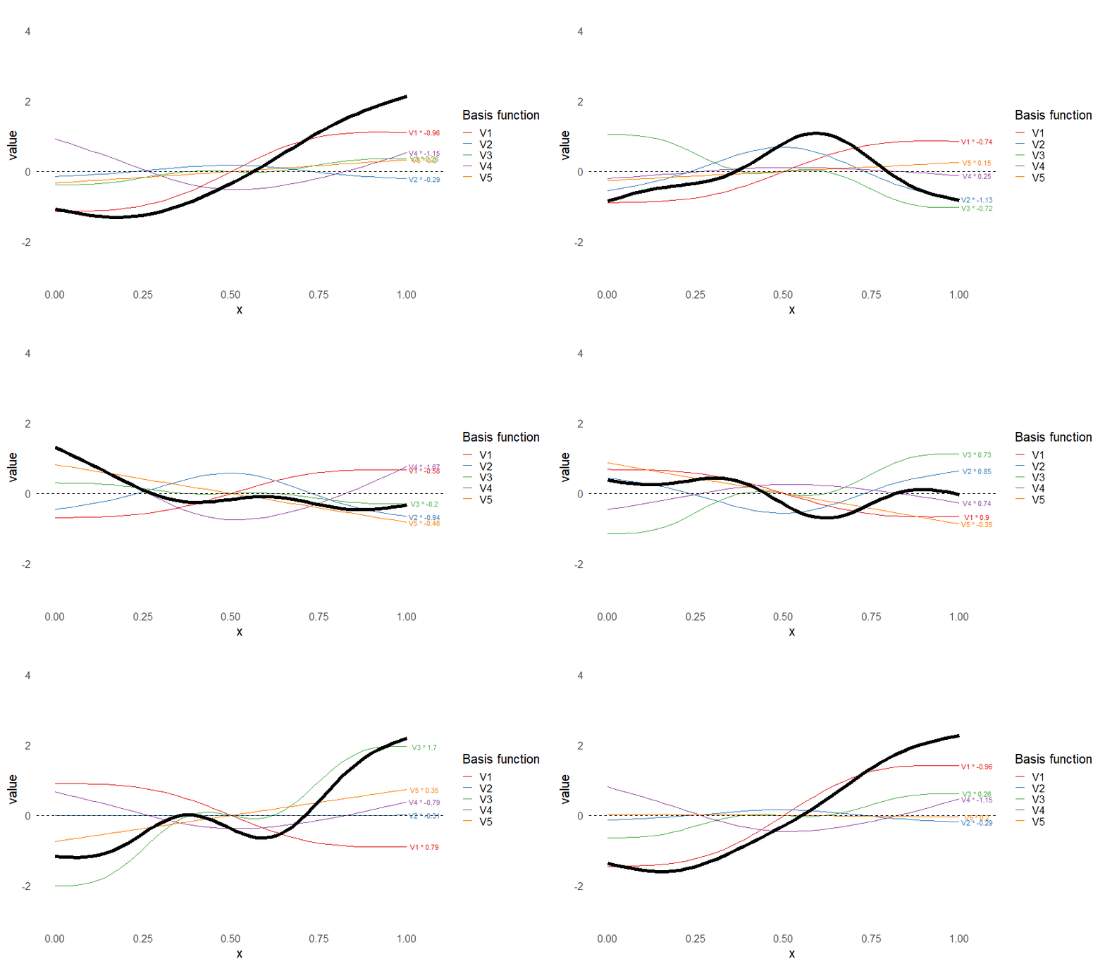
This leads to some very flexible functions!

Shiny app!

Click here

Basis-penalty smoothers

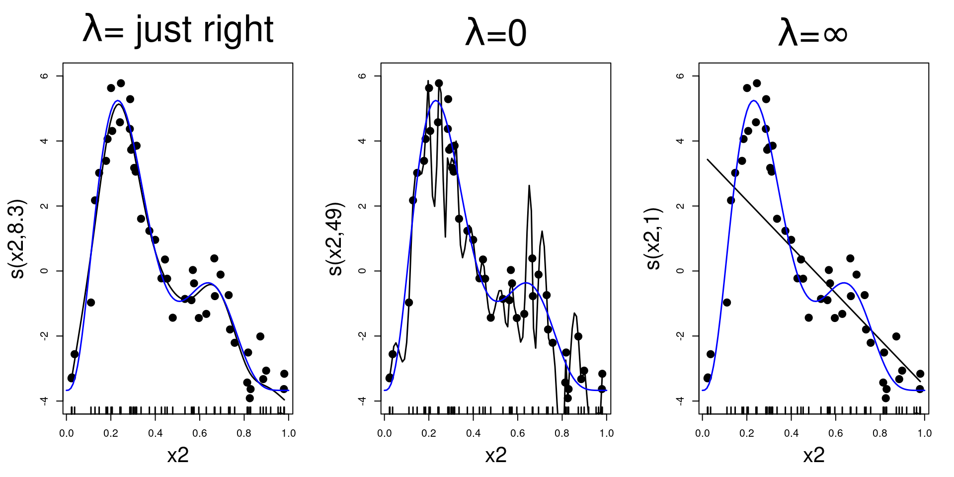
• How do we avoid overfitting?
• Measure wigglyness, then penalise!

\[ \lambda \int_\mathbb{R} \left( \frac{\partial^2 s(x)}{\partial x^2}\right)^2 \text{d}x\\ \]

where \(\lambda\) is a smoothing parameter

Basis-penalty smoothers

• How do we avoid overfitting?
• Measure wigglyness, then penalise!

Effective degrees of freedom

• We need to set number of basis functions (\(k\))
• This sets the maximum complexity
• But we penalize so there is some shrinkage in the coefficients
• How many basis functions did we effectively use?
• effective degrees of freedom – EDF

Effective degrees of freedom

Putting that in a model

\[ \mathbb{E}(Y_i) = g^{-1}\left[\beta_0 + \sum_j s_j(x_{ij})\right] \]

• \(Y_i \sim\) some (extended?) exponential family
• \(g\) is a link function
• \(\beta_0\) is an intercept
• \(s_j(x_{ij})\) are smooths!

Okay, what about practical stuff…

Fitting GAMs in R

• Lots of packages exist: gam, mgcv, R-INLA, brms, gamlss
• Here we’ll focus on mgcv
  • R package, by Simon Wood (Edinburgh)
  • Uses familiar glm()-type syntax
  • Recommended (ships with R)
  • Very fast (and parallelisable)

The data we’re going to look at

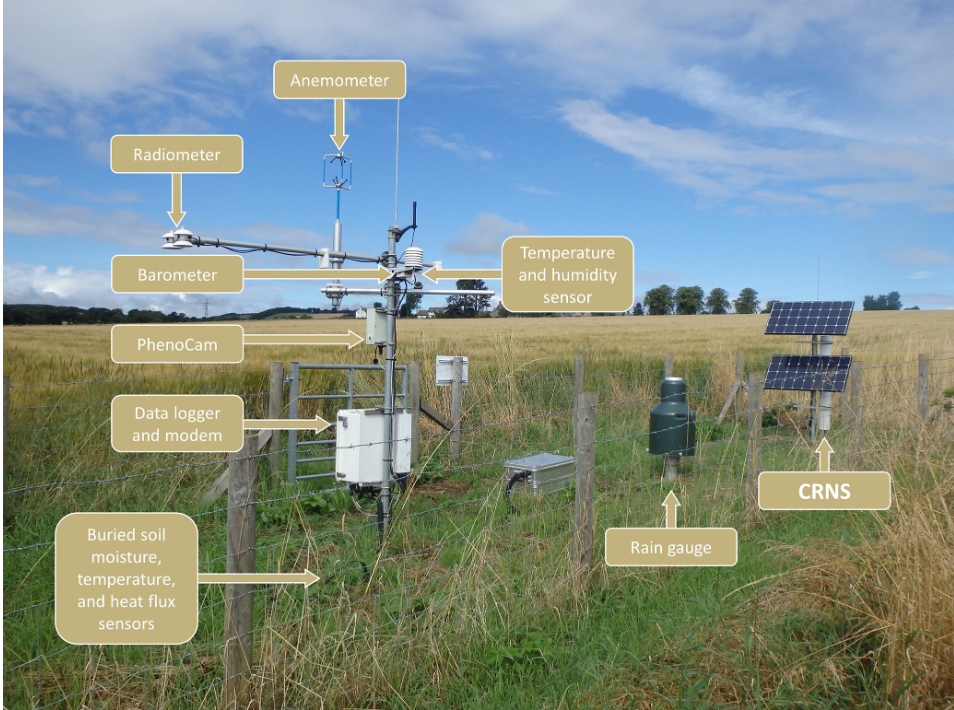
UKCEH data: COSMOS-UK https://cosmos.ceh.ac.uk/

Dataset from: https://catalogue.ceh.ac.uk/documents/5060cc27-0b5b-471b-86eb-71f96da0c80f

COSMOS-UK

Using ✨cosmic rays✨ to measure moisture

COSMOS-UK data

# A tibble: 127,228 × 16
  SITE_ID SITE_NAME  LONGITUDE LATITUDE NORTHING EASTING ALTITUDE LAND_COVER    
  <fct>   <chr>          <dbl>    <dbl>    <dbl>   <dbl>    <dbl> <fct>         
1 ALIC1   Alice Holt    -0.858     51.2   139985  479950       80 Broadleaf woo…
2 ALIC1   Alice Holt    -0.858     51.2   139985  479950       80 Broadleaf woo…
3 ALIC1   Alice Holt    -0.858     51.2   139985  479950       80 Broadleaf woo…
4 ALIC1   Alice Holt    -0.858     51.2   139985  479950       80 Broadleaf woo…
5 ALIC1   Alice Holt    -0.858     51.2   139985  479950       80 Broadleaf woo…
6 ALIC1   Alice Holt    -0.858     51.2   139985  479950       80 Broadleaf woo…
7 ALIC1   Alice Holt    -0.858     51.2   139985  479950       80 Broadleaf woo…
8 ALIC1   Alice Holt    -0.858     51.2   139985  479950       80 Broadleaf woo…
# ℹ 127,220 more rows
# ℹ 8 more variables: SOIL_TYPE <fct>, DATE_TIME <date>, PRECIP <dbl>,
#   SNOW_DEPTH <dbl>, COSMOS_VWC <dbl>, ndate <dbl>, month <dbl>, year <dbl>

COSMOS-UK data

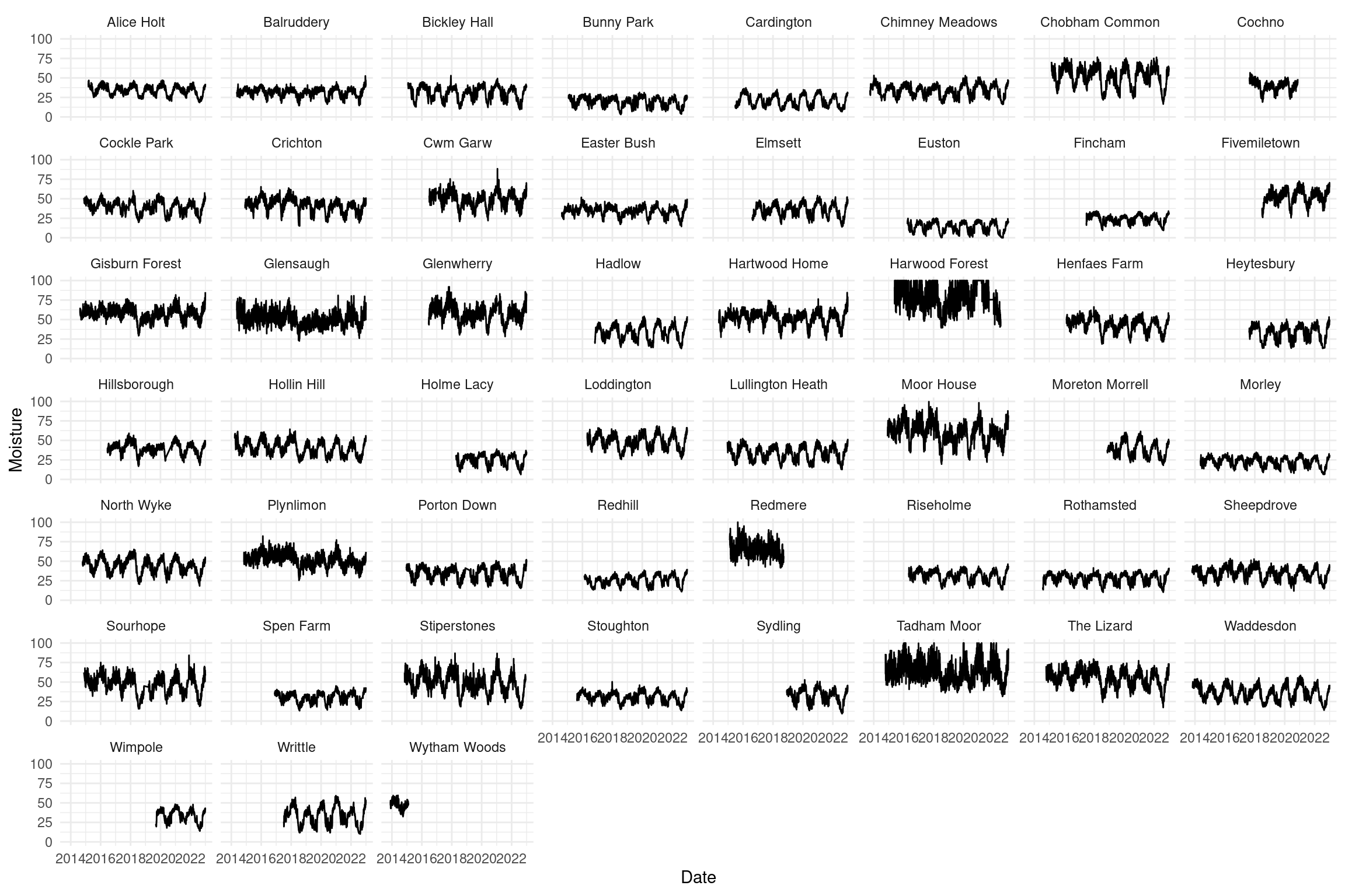
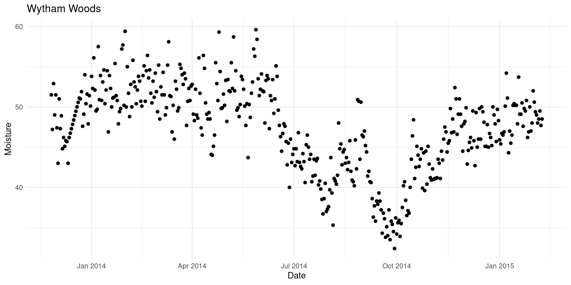
Let’s try to fit a model to the soil data

• Simple: predict moisture as a function of day (for one site)
• Ignore some data structure (for now)

The model

• Denote:
  • day by \(t\)
  • moisture on day \(t\) is \(m_{t}\)

• Assume \(m_{t} \sim N(\mu_t, \sigma)\)

• Smooth effect of day: \(s(t)\)

The model

• Denote:
  • day by \(t\)
  • moisture on day \(t\) is \(m_{t}\)

• Assume \(m_{t} \sim N(\mu_t, \sigma)\)

• Smooth effect of day: \(s(t)\)

Our model is then: \[ \mathbb{E}(\mu_t) = \beta_0 + s(t) \]

Fitting a model with gam

• If we know how to use glm, we know how to use gam
• We need a formula and some data
• We can denote smooths with s()
  • e.g., s(x)

library(mgcv)
wwoods <- subset(all_sites, SITE_NAME=="Wytham Woods")

b <- gam(COSMOS_VWC ~ s(ndate), data=wwoods, method="REML")

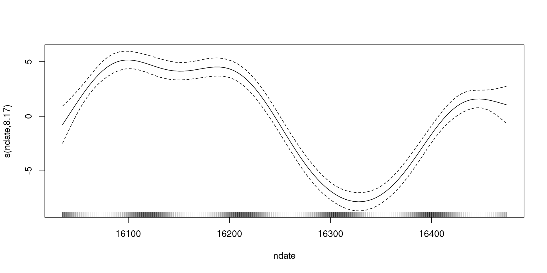
What did that do?

summary(b)

Family: gaussian 
Link function: identity 

Formula:
COSMOS_VWC ~ s(ndate)

Parametric coefficients:
            Estimate Std. Error t value Pr(>|t|)    
(Intercept)  47.3525     0.1524   310.7   <2e-16 ***
---
Signif. codes:  0 '***' 0.001 '**' 0.01 '*' 0.05 '.' 0.1 ' ' 1

Approximate significance of smooth terms:
           edf Ref.df    F p-value    
s(ndate) 8.167  8.812 95.1  <2e-16 ***
---
Signif. codes:  0 '***' 0.001 '**' 0.01 '*' 0.05 '.' 0.1 ' ' 1

R-sq.(adj) =  0.656   Deviance explained = 66.3%
-REML = 1150.5  Scale est. = 10.218    n = 440

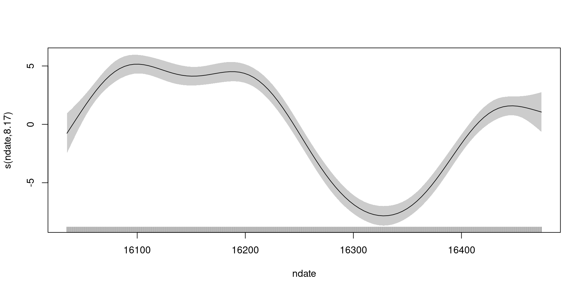
What did that do?

plot(b)

What did that do?

plot(b, shade=TRUE)

Was the smooth wiggly enough?

gam.check(b)

Method: REML   Optimizer: outer newton
full convergence after 7 iterations.
Gradient range [-3.367285e-07,8.300716e-08]
(score 1150.533 & scale 10.2183).
Hessian positive definite, eigenvalue range [3.13693,219.0595].
Model rank =  10 / 10 

Basis dimension (k) checking results. Low p-value (k-index<1) may
indicate that k is too low, especially if edf is close to k'.

           k'  edf k-index p-value    
s(ndate) 9.00 8.17     0.5  <2e-16 ***
---
Signif. codes:  0 '***' 0.001 '**' 0.01 '*' 0.05 '.' 0.1 ' ' 1

Let’s double k

Family: gaussian 
Link function: identity 

Formula:
COSMOS_VWC ~ s(ndate, k = 20)

Parametric coefficients:
            Estimate Std. Error t value Pr(>|t|)    
(Intercept)  47.3525     0.1289   367.4   <2e-16 ***
---
Signif. codes:  0 '***' 0.001 '**' 0.01 '*' 0.05 '.' 0.1 ' ' 1

Approximate significance of smooth terms:
           edf Ref.df     F p-value    
s(ndate) 17.43  18.68 71.43  <2e-16 ***
---
Signif. codes:  0 '***' 0.001 '**' 0.01 '*' 0.05 '.' 0.1 ' ' 1

R-sq.(adj) =  0.754   Deviance explained = 76.4%
-REML = 1099.9  Scale est. = 7.3089    n = 440

What do our models look like?

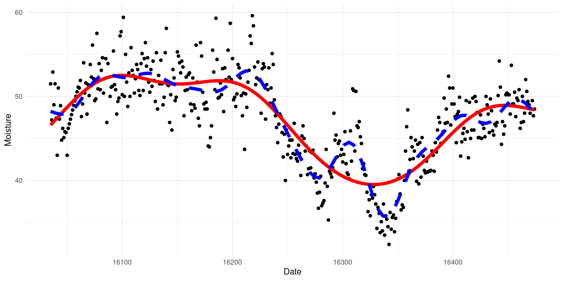
(you’ll learn how to do this later!)

Recap

• GAMs are GLMs with extra wiggles
• We use basis functions to model flexible effects
• We need to penalize our fit to avoid overfitting
• gam() fits a GAM
• summary() gives us information about the fit
• plot() makes basic plots